The hardware and bandwidth for this mirror is donated by dogado GmbH, the Webhosting and Full Service-Cloud Provider. Check out our Wordpress Tutorial.
If you wish to report a bug, or if you are interested in having us mirror your free-software or open-source project, please feel free to contact us at mirror[@]dogado.de.
Our package uses state-of-the-art state-space models to facilitate the modeling and forecasting of financial intraday signals. It currently offers a univariate model for intraday trading volume, with new features on intraday volatility and multivariate models in development. It is a valuable tool for anyone interested in exploring intraday, algorithmic, and high-frequency trading.
The package can be installed from GitHub:
# install development version from GitHub
devtools::install_github("convexfi/intradayModel")
Please cite intradayModel in publications:
citation("intradayModel")To get started, we load our package and sample data: the 15-minute intraday trading volume of AAPL from 2019-01-02 to 2019-06-28, covering 124 trading days. We use the first 104 trading days for fitting, and the last 20 days for evaluation of forecasting performance.
library(intradayModel)
data(volume_aapl)
volume_aapl[1:5, 1:5] # print the head of data
#>          2019-01-02 2019-01-03 2019-01-04 2019-01-07 2019-01-08
#> 09:30 AM   10142172    3434769   20852127   15463747   14719388
#> 09:45 AM    5691840   19751251   13374784    9962816    9515796
#> 10:00 AM    6240374   14743180   11478596    7453044    6145623
#> 10:15 AM    5273488   14841012   16024512    7270399    6031988
#> 10:30 AM    4587159   18041115    8686059    7130980    5479852

volume_aapl_training <- volume_aapl[, 1:104]
volume_aapl_testing <- volume_aapl[, 105:124]
Next, we fit a univariate state-space model using
fit_volume() function.
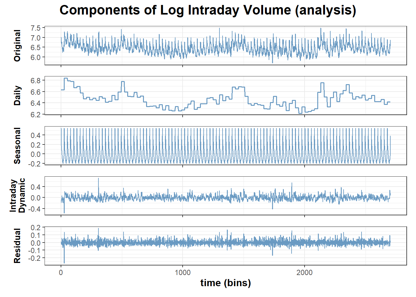
model_fit <- fit_volume(volume_aapl_training)Once the model is fitted, we can analyze the hidden components of any
intraday volume based on all its observations. By calling
decompose_volume() function with
purpose = "analysis", we obtain the smoothed daily,
seasonal, and intraday dynamic components. It involves incorporating
both past and future observations to refine the state estimates.
analysis_result <- decompose_volume(purpose = "analysis", model_fit, volume_aapl_training)

# visualization
plots <- generate_plots(analysis_result)
plots$log_components
To see how well our model performs on new data, we call
forecast_volume() function to do one-bin-ahead forecast on
the testing set.
forecast_result <- forecast_volume(model_fit, volume_aapl_testing)

# visualization
plots <- generate_plots(forecast_result)
plots$original_and_forecast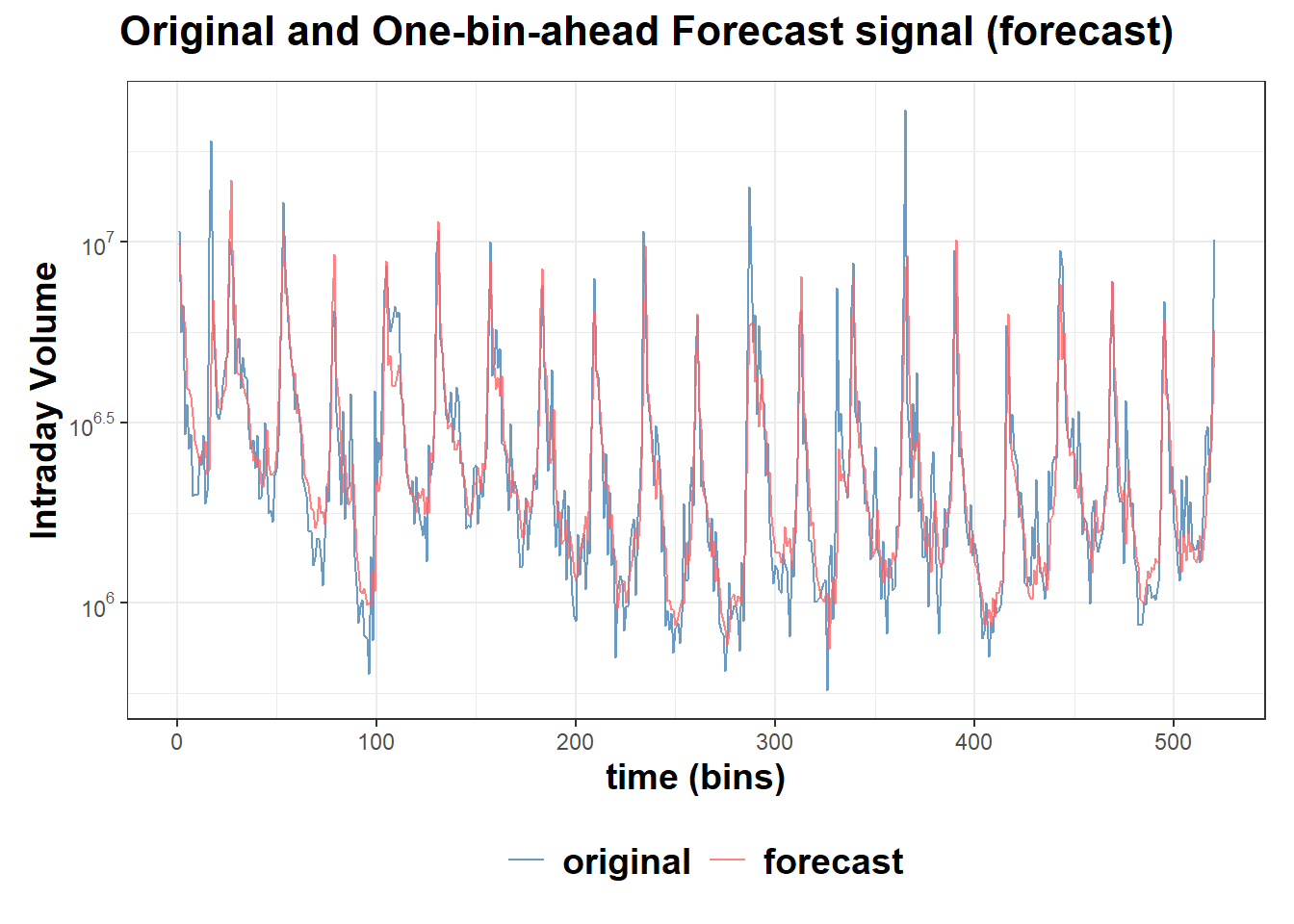
We welcome all sorts of contributions. Please feel free to open an issue to report a bug or discuss a feature request.
If you make use of this software please consider citing:
Package: GitHub
Vignette: GitHub-vignette.
These binaries (installable software) and packages are in development.
They may not be fully stable and should be used with caution. We make no claims about them.
Health stats visible at Monitor.