

The hardware and bandwidth for this mirror is donated by dogado GmbH, the Webhosting and Full Service-Cloud Provider. Check out our Wordpress Tutorial.
If you wish to report a bug, or if you are interested in having us mirror your free-software or open-source project, please feel free to contact us at mirror[@]dogado.de.
insectecol (Insect Ecology Data Analysis Toolkit) is a collection of analytical tools for insect ecology research. It currently ships four modules:
lifeTable_analyze() for data already loaded in R, batch
function lifeTable_calculate() for csv files on disk.
Validates raw csv data, computes the cohort size (N), mean fecundity
(F), age-stage survival rates (s_xj), age-specific survival (l_x),
age-specific fecundities (F_xj, m_x), life expectancy (e_x) and the
derived population parameters (net reproductive rate R0, intrinsic and
finite rates of increase r and lambda, mean generation time T), draws
the age-stage survival curves and exports all tabular results and plots
to Excel in a single run. Fast batch processing of multi-group datasets
is supported.lc50_analyze() for data already loaded in R, one-step batch
functions lc50_export_auto() (Excel tables) and
lc50_export_plot_auto() (figures) for csv files on disk.
Estimates lethal concentrations by the traditional and the weighted
(improved) linear regression methods and by probit analysis, with Abbott
correction, 95% confidence intervals and chi-square goodness-of-fit
tests. The lethal proportion can be set freely (25%, 50%, 70%, 90%, …),
so any LC value such as the LC25, LC70 or LC90 can be computed - not
only the LC50. Regression plots and tables are exported to Excel.gdd_analyze() for data already loaded in R (column vectors,
a data frame, or csv/xlsx file(s)). Estimates the developmental
threshold temperature C and the effective accumulated temperature K by
the linear degree-day law (T = C + K·V, fitted with the exact standard
errors of the linear model), fits six common nonlinear
temperature-dependent development models (Logan-6, Lactin 1995,
Briere-1/2 1999, Wang-7) and selects the best per group by AICc
(model = "auto"), with a linear-range check that warns when
the rate declines at high temperatures. Publication figures use a serif
font by default (Times New Roman on Windows; Chinese characters fall
back to SimSun automatically) and can be exported at any physical size
and resolution. Further tools: prediction (gdd_predict()),
pairwise group comparison (gdd_compare()), degree-day
accumulation from daily Tmin/Tmax (gdd_daily()), deriving
data from a life-table csv csv/xlsx export (gdd_export())
and png export (gdd_export_plot()).emergence_analyze() for data already loaded
in R (column vectors, a data frame, or csv/xlsx file(s)). Turns one
field survey of the population stage structure (e.g. a dissected-sample
count of pupal grades) into the projected dates of the 16% / 50% / 84%
emergence quantiles - the beginning, peak and end of the adult emergence
period - by the classic Chinese stage-grading method (分龄分级推算法),
and optionally projects the larval hatch dates from the pre-oviposition
period and the egg duration. Quantiles outside the surveyed range are
extrapolated with an explicit warning, English and Chinese column
headers are auto-detected, publication figures follow the same
serif-font conventions as the degree-day module, and tables and figures
are exported with emergence_export() /
emergence_export_plot().Each module has a main function for analysing data that are already loaded in R (a data frame or plain vectors) and a one-step batch function for processing csv files on disk:
| Module | Main function (data in R) | One-step batch (csv on disk) |
|---|---|---|
| Life table | lifeTable_analyze() |
lifeTable_calculate() |
| Bioassay | lc50_analyze() |
lc50_export_auto() (tables),
lc50_export_plot_auto() (figures) |
| Degree-day | gdd_analyze() |
gdd_analyze(path = ...) also reads files/folders,
gdd_export() writes the tables,
gdd_export_plot() the figure |
| Emergence period | emergence_analyze() |
emergence_analyze(path = ...) also reads files/folders,
emergence_export() writes the tables,
emergence_export_plot() the figure |
The main functions assemble the data, compute everything and
optionally build the plots, but never write to disk - export is handled
separately by lifeTable_export(),
lc50_export() and lc50_export_plot(), so the
results stay fully customisable inside R.
For full control, every module can also be driven step by step
(lifeTable_read() ->
lifeTable_calculate_all() ->
lifeTable_plot() -> lifeTable_export(), and
lc50_read() -> lc50_calculate() ->
lc50_plot() -> lc50_export() /
lc50_export_plot()); see the function reference below.
Planned extensions include more insect ecology indicators, such as the median lethal temperature/time (LT50).
# from CRAN (once accepted)
install.packages("insectecol")

# development version from GitHub
# install.packages("devtools")
devtools::install_github("SeaGhost-0/insectecol")library(insectecol)
# example data shipped with the package
f <- system.file("extdata", "lifetable_example.csv", package = "insectecol")
d <- read.csv(f)
# analyse straight from the columns of the loaded data frame
out <- lifeTable_analyze(
stages = d[2:8], # one column per immature stage
adult_days = d$Adult, # adult survival days
sex = d$gender, # "F" / "M" / "N" (died before adult)
oviposition = d[, 11:17], # daily oviposition of the females
file_name = "Example"
)
out$results$N # cohort size
out$results$R0 # net reproductive rate
out$results$lambda # finite rate of increase
# survival analysis only: skip the reproduction-related parameters
out2 <- lifeTable_analyze(
stages = d[2:8],
adult_days = d$Adult,
sex = d$gender,
fecundity = FALSE # no oviposition data required
)
# with the age-stage survival curve (a ggplot object)
out3 <- lifeTable_analyze(
stages = d[2:8], adult_days = d$Adult, sex = d$gender,
oviposition = d[, 11:17], plot = TRUE
)
print(out3$plot)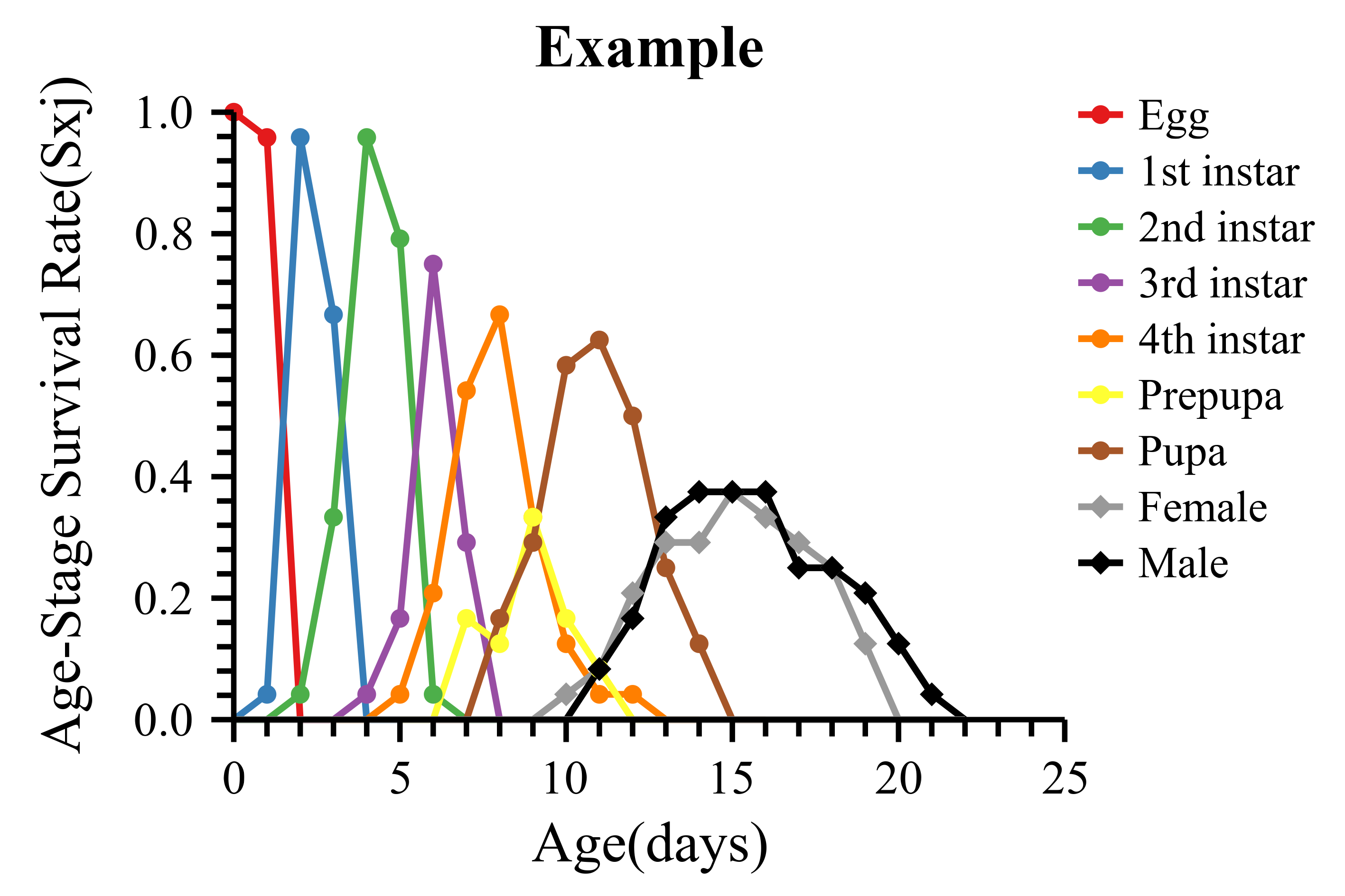
To batch-process csv files on disk instead (each csv gets its own
Excel workbook with all results and the survival curve; an additional
all.xlsx summarises every file):
lifeTable_calculate("path/to/lifetable_data")library(insectecol)
# three parallel vectors - no csv file involved
conc <- c(0, 1.5, 3, 6, 12, 24)
tested <- c(120, 60, 60, 60, 60, 60)
dead <- c(7, 9, 18, 32, 48, 57)
out <- lc50_analyze(
concentration = conc,
tested = tested,
dead = dead,
name = "trial1",
method = "all", # traditional + improved + probit in one call
lc = 0.5 # LC50; any proportion works (e.g. 0.9 = LC90)
)
out$results$summary_df # estimate, 95% CI, slope, chi-square, ...
# ... or straight from the example csv shipped with the package
f <- system.file("extdata", "lc50_example.csv", package = "insectecol")
out_csv <- lc50_analyze(lc50_read(f), method = "all")
out_csv$results$summary_df
# with the regression plot (a named list of ggplot objects)
out2 <- lc50_analyze(
concentration = conc, tested = tested, dead = dead,
name = "trial1", method = "probit", plot = TRUE
)
print(out2$plot$trial1)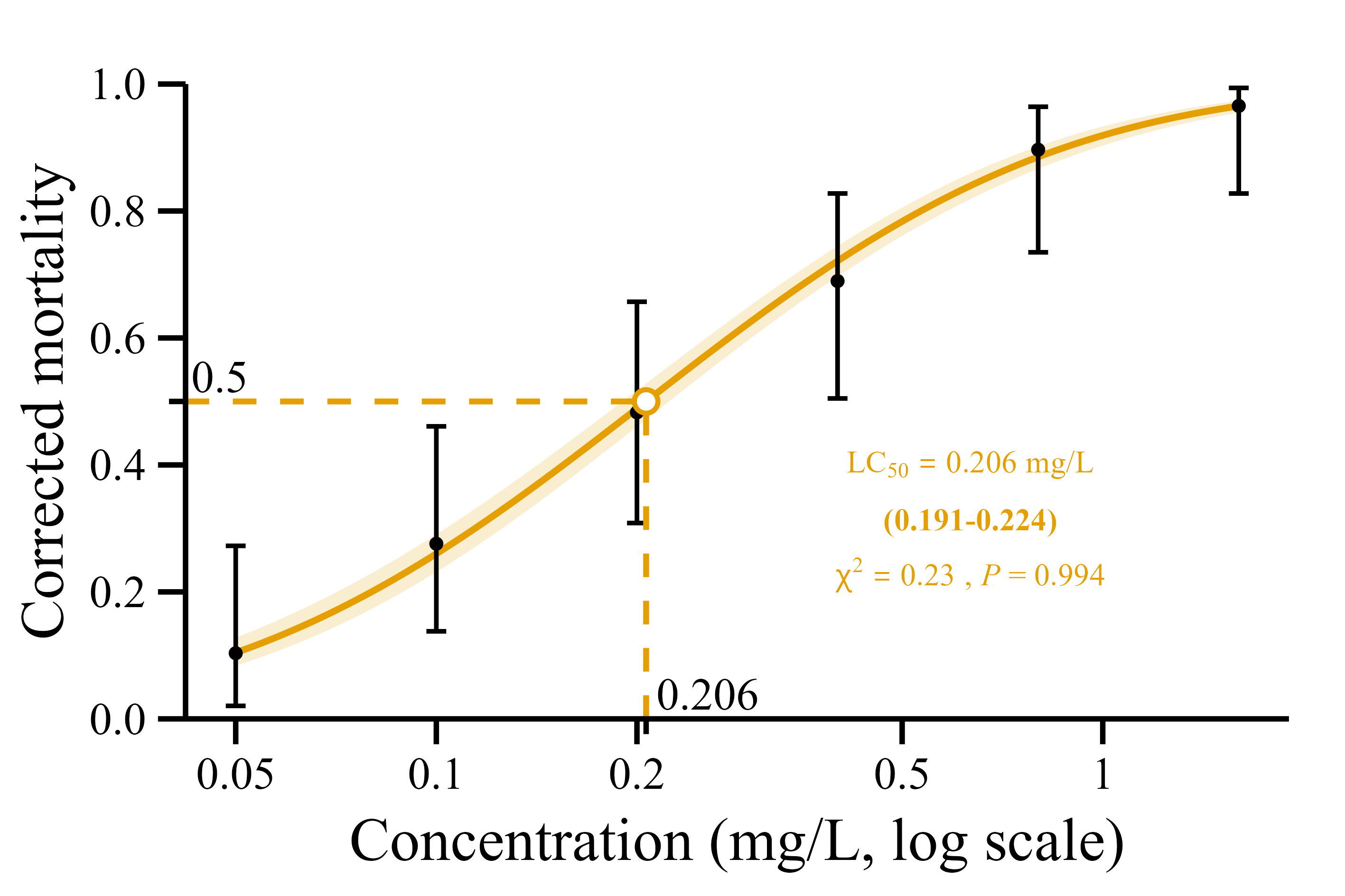
To batch-process csv files on disk instead (one xlsx / one tiff per
csv, written next to the raw data; non-default settings are appended to
the file names, e.g. LB_48_LC90_probit.xlsx):
lc50_export_auto("path/to/bioassay_data", method = "probit")
lc50_export_plot_auto("path/to/bioassay_data", method = "probit")library(insectecol)
# example data shipped with the package
f <- system.file("extdata", "gdd_example.csv", package = "insectecol")
d <- read.csv(f)
# analyse straight from the columns of the loaded data frame
out <- gdd_analyze(
temp = d$temp, # temperature (deg C)
duration = d$duration, # mean developmental duration (days)
group = d$stage # optional grouping column (e.g. life stage)
)
out$fit$results # C, K, SE and 95% CI per group (linear degree-day law)
summary(out$fit) # detailed coefficient tables
# nonlinear models with AICc selection and a publication png
out2 <- gdd_analyze(temp = d$temp, duration = d$duration, group = d$stage,
model = "auto", # best of six models per group
plot = TRUE, plot_file = "gdd.png",
plot_units = "cm", plot_width = 16, plot_res = 300)
out2$fit$comparison # full model comparison table, best flag included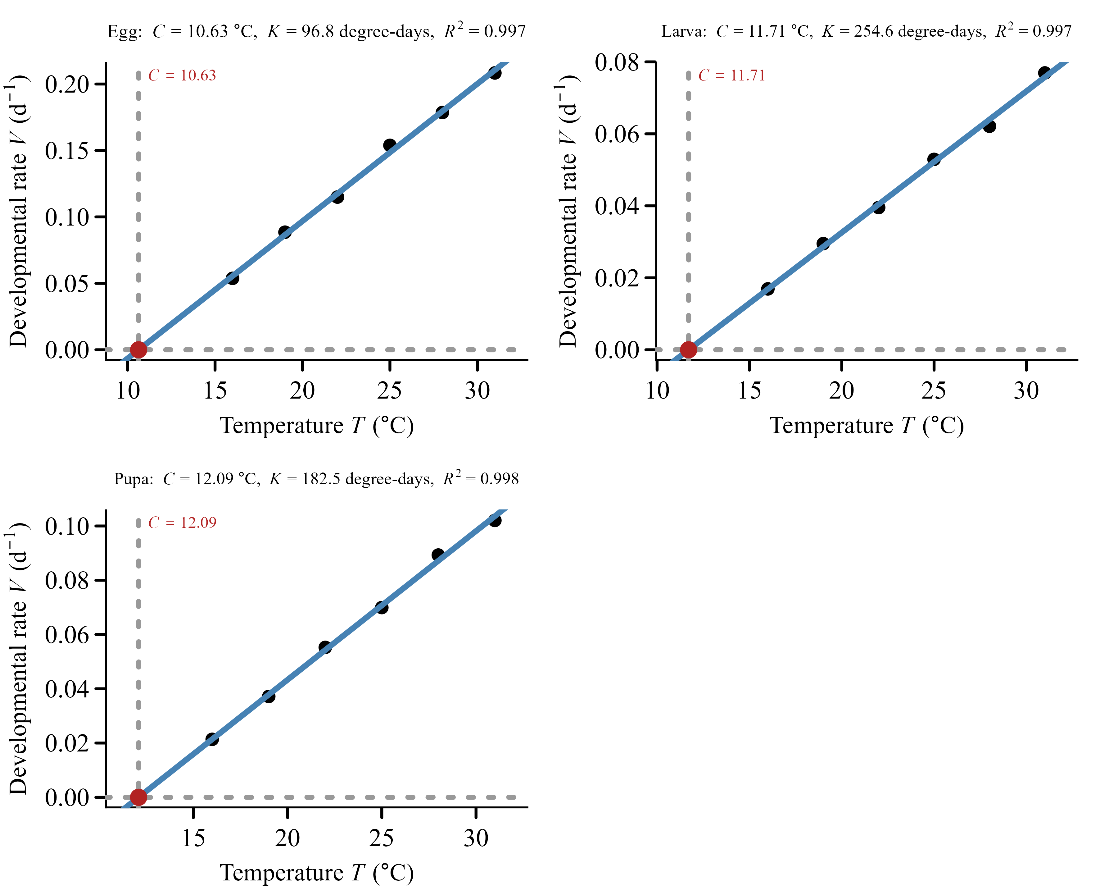
Without plot_file the figure is drawn on the current
device and stays fully customisable via gdd_plot() (custom
titles/axis labels, named per-group titles, family font).
The exported png size is physical (plot_units =
"in"/"cm"/"px") so
plot_res only changes the sharpness and the recorded dpi,
never the layout.
For batch csv processing, gdd_analyze(path = "folder")
reads every csv/xlsx in a folder (combined with a
source_file column), and gdd_export() writes
the result tables (gdd_export_plot() the figure):
out3 <- gdd_analyze(path = "path/to/gdd_data", model = "auto")
gdd_export(out3$fit, file = "gdd_results.csv")
gdd_export_plot(out3$fit, file = "gdd.png")library(insectecol)
# example data shipped with the package: one survey of the pupal
# grade structure (Tianyang overwintering generation, 40 individuals)
f <- system.file("extdata", "emergence_example.csv", package = "insectecol")
d <- read.csv(f)
# stage count days # days = days from this stage to
# Pupal exuviae 2 0 # adult eclosion at the current
# Pupa 7 3 2 # temperature (most developed first)
# ...
# analyse straight from the columns of the loaded data frame
out <- emergence_analyze(
stage = d$stage, count = d$count, days = d$days,
survey_date = "2026-03-20"
)
out$fit$predictions # dates of the beginning (16%), peak (50%)
# and end (84%) of the emergence period
predict(out$fit, c(0.25, 0.75)) # arbitrary quantiles
summary(out$fit) # full cumulative table
# larval hatch: eclosion + pre-oviposition period + egg duration
out2 <- emergence_analyze(data = d, survey_date = "2026-03-20",
pre_ovip = 3, egg_days = 10,
plot = TRUE, plot_file = "emergence.png")
out2$fit$predictions$hatch_date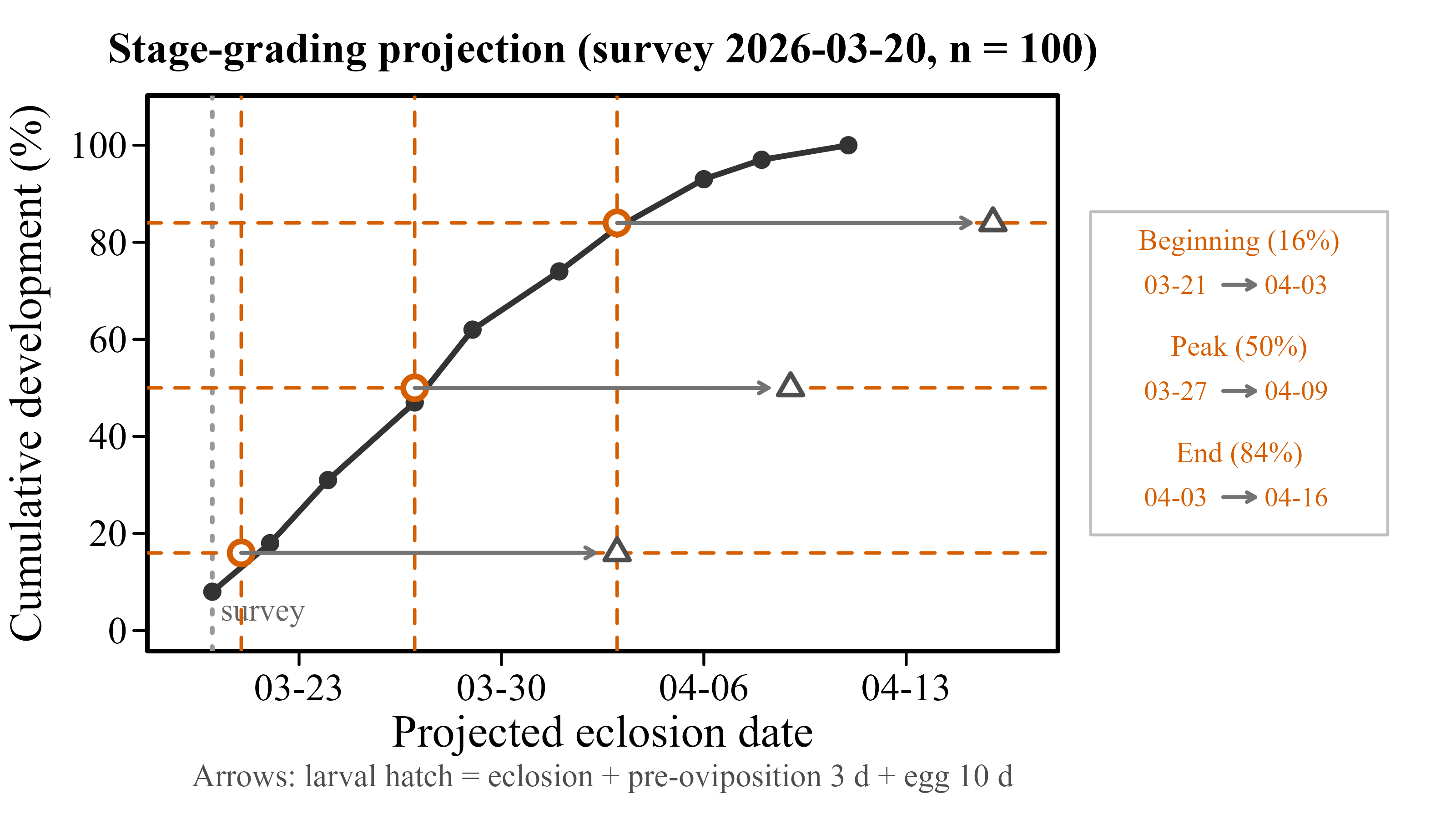
The three quantile dates are interpolated on the cumulative
development curve built from the survey; a survey that misses stages
simply renormalises the shares, while a quantile below the share of the
most developed stage (partly eclosed before the survey) is extrapolated
backwards with an explicit warning. Tables are exported with
emergence_export(fit, file = "emergence_results.csv"), the
figure with
emergence_export_plot(fit, file = "emergence.png").
Four example csv files ship with the package in
inst/extdata/; the examples in this README and in the help
pages are built on them:
system.file("extdata", "lifetable_example.csv", package = "insectecol")      # life table
system.file("extdata", "lc50_example.csv", package = "insectecol")     # bioassay
system.file("extdata", "gdd_example.csv", package = "insectecol")  # degree-day
system.file("extdata", "emergence_example.csv",
            package = "insectecol")                                # emergence
Example.csv - life table data in the csv template: one
row per individual with the ID, the days spent in each of
the seven immature stages (egg, four larval instars, prepupa, pupa), the
adult survival days, the sex
(F/M/N) and the daily oviposition
of the females.bioassay.csv - bioassay data: one row per concentration
group with the columns Concentration (0 = control group for
the Abbott correction), Tested and Dead.gdd_example.csv - degree-day data: one row per
temperature with the columns temp (deg C),
duration (mean developmental duration in days) and
stage (the grouping column).
inst/extdata/gdd_batch/ additionally ships one file per
temperature for the batch mode.emergence_example.csv - emergence-period survey data
(the Tianyang overwintering-generation case): one row per stage with the
columns stage, count (individuals in that
stage) and days (average days from that stage to adult
eclosion).The file layouts are described in detail under Data formats.
One row per individual. If the sex column is at position
n:
| Column | Content |
|---|---|
| 1 | individual ID (header ID) |
| 2 … n-2 | days spent in each immature stage (egg, instars, prepupa, pupa) |
| n-1 | adult survival days |
| n | sex: F, M or N (died before
the adult stage); header gender |
| n+1 … | daily oviposition of the females (one column per day) |
The first line must contain the stage names as headers. The sex column is located automatically, and the file encoding is detected automatically (UTF-8 and GBK are both supported).
One row per concentration group (replicates = repeated concentration values):
| Column | Content |
|---|---|
Concentration |
the concentration (0 = control group, used for the Abbott correction) |
Tested |
number of insects tested |
Dead |
number of dead insects |
Headers are matched loosely, so a header like
Concentration (mg/L) is recognised as well. UTF-8 (with
BOM) and GBK encodings are supported.
One row per temperature (long format):
| Column | Content |
|---|---|
| temperature | rearing temperature in deg C (e.g. temp,
temperature, T, 温度) |
| duration | mean developmental duration in days (e.g. duration,
days, D, 发育天数,
历期) |
| group (optional) | grouping variable, e.g. the life stage |
The temperature and duration columns are auto-detected (English and
Chinese headers are recognised); ambiguous files accept explicit
temp_col / duration_col. UTF-8 (with BOM) and
GBK encodings are supported; the csv delimiter (,
; tab) is auto-detected, and xlsx files are read via
readxl.
One row per stage, ordered most-developed-first (the rows are sorted
by days internally anyway):
| Column | Content |
|---|---|
| stage | stage name, e.g. the pupal grade (stage,
grade, 虫态, 阶段) |
| count or percent | individuals observed in that stage, or its share
(count, n, 数量,
虫数 / percent, 占比) |
| days | average days from that stage to adult eclosion (days,
天数, 历期, 距羽化天数) |
The columns are auto-detected (English and Chinese headers are
recognised); ambiguous files accept explicit stage_col /
count_col / percent_col /
days_col. Exactly one of count / percent is used (count
wins with a message when both are present). UTF-8 (with BOM) and GBK
encodings are supported; the csv delimiter is auto-detected, and xlsx
files are read via readxl.
| Function | Purpose |
|---|---|
lifeTable_analyze() |
main function - analyse data in R (build + compute + optional plot) |
lifeTable_build() |
build a life_table object from user-supplied
columns |
lifeTable_read() |
read and validate a life table csv file |
lifeTable_calculate() |
batch: analyse every csv in a folder and export to Excel |
lifeTable_calculate_all() |
all parameters of one life_table object |
calc_N(), calc_F(),
calc_sxj(), calc_lx(),
calc_fxj(), calc_mx(), calc_ex(),
calc_R0(), calc_r(),
calc_lambda(), calc_T() |
individual indicators |
lifeTable_plot() |
age-stage survival rate curves |
lifeTable_export() |
export one analysis to Excel |
lifeTable_check(), get_stage_names(),
default_stage_names() |
helpers |
| Function | Purpose |
|---|---|
lc50_analyze() |
main function - analyse data in R (build + compute + optional plots) |
lc50_read() |
read bioassay csv file(s) |
lc50_calculate() |
compute the LC values; several methods (or "all") in
one call |
lc50_plot() |
regression plots |
lc50_export() |
export results to Excel |
lc50_export_plot() |
export figures |
lc50_export_auto() |
one-step batch: csv file(s) -> Excel workbook(s) |
lc50_export_plot_auto() |
one-step batch: csv file(s) -> tiff figure(s) |
check_path_type() |
path helper (folder / csv file) |
| Function | Purpose |
|---|---|
gdd_analyze() |
main function - read/check/fit/plot in one call (column vectors, data frame, or path) |
gdd_read() |
read a gdd csv/xlsx file or a folder of them (batch) |
gdd_check() |
validate the data; linear-range check (rate decline warning) |
gdd_calc() |
fit one model per group, or model = "auto" (AICc
selection) |
gdd_compare() |
pairwise comparison of the groups |
gdd_plot() |
fitted line/curve per group (custom titles, font family, size/dpi) |
gdd_predict() |
predicted developmental duration at given temperatures |
gdd_daily() |
degree-day accumulation from daily Tmin/Tmax (avg / triangle method) |
gdd_export() |
export the result tables to csv/xlsx |
gdd_export_plot() |
export the fitted line/curve figure as png |
| Function | Purpose |
|---|---|
emergence_analyze() |
main function - read/compute/plot in one call (column vectors, data frame, or path) |
emergence_read() |
read an emergence csv/xlsx file or a folder of them (batch) |
emergence_calc() |
cumulative development + quantile dates from a survey table |
emergence_export() |
export the prediction and stage tables to csv/xlsx |
emergence_export_plot() |
export the projection figure as png |
print() / summary() /
predict() / plot() |
S3 methods for the emergence object
(predict(fit, p) interpolates arbitrary quantiles) |
Figures and fonts
lc50_plot() falls back to plain text
when the unit contains Chinese, so that the unit is set in the CJK font
like every other label. The percentage is then written LC50
instead of with a subscript, because plotmath can only draw a whole
expression with one font.plot = TRUE in lifeTable_analyze(),
lc50_analyze(), emergence_analyze() and
gdd_analyze() now always writes the figure: with no
plot_file it goes to the working directory under a default
name (<file_name>_plot.png,
LC50_<name>.png, emergence_plot.png or
gdd_plot.png), and a plot_file without an
extension is treated as a folder - created when missing - with the
figure written inside it. Previously the figure was only returned and
ggsave() stopped on a folder path.plot_file extension (png/tiff/jpeg written by
ragg when available).Examples
\dontrun replaced by \donttest throughout:
every example can be run by the user, and only the parts that write a
workbook - which take well over five seconds - are skipped by
R CMD check.Internal changes
lifeTable_analyze(plot = TRUE) are
now written through the same device machinery as the other functions:
bitmaps go through ragg (per-glyph font fallback) and
vector formats through showtext, so a
plot_file pointing at a pdf or svg works as well.windowsFonts(), and the bundled-font fallback registers its
metrics with the vector devices too - the package builds and checks
cleanly on Linux and macOS.systemfonts added to Imports (the package
ragg draws and measures text with); it supplies the
per-character widths used to split a mixed label into runs.Version 1.1.1 adds the emergence-period module, standardises the
function naming across all modules
(<module>_<verb> with the same verbs
everywhere, see below) and removes the no-longer-needed
gdd_from_lifetable() bridge.
Function naming unified across modules
<module>_<verb> scheme of the newer modules,
and every module uses the same word for the same action -
*_analyze() (main entry), *_read() (file
intake), *_plot() (figures), *_export()
(tables to csv/xlsx), *_export_plot() (figures to
png/tiff). Renamed: read_life_table() ->
lifeTable_read(), build_life_table() ->
lifeTable_build(), plot_sxj() ->
lifeTable_plot(), check_life_table() ->
lifeTable_check(), save_results() ->
lifeTable_export(), read_lc50() ->
lc50_read(), plot_lc50() ->
lc50_plot(), save_lc50() ->
lc50_export(), save_lc50_plot() ->
lc50_export_plot(), save_lc50_auto() ->
lc50_export_auto() and save_lc50_plot_auto()
-> lc50_export_plot_auto(). The old names are removed
(the previous release had essentially no users); the low-level indicator
helpers (calc_N(), calc_R0(), …) keep their
short names.gdd_export_plot() and
emergence_export_plot(): export the figure of an existing
fit as png at any time (the standalone counterpart of
plot_file = in the two *_analyze() functions,
which now reuse them internally).plot_file png export added to all four main functions:
the life-table (lifeTable_analyze()) and bioassay
(lc50_analyze()) main functions now also accept
plot_file (with
plot_width/plot_height/plot_units/plot_res),
so one call goes from raw data to the finished figure file in every
module.gdd_from_lifetable(): the raw-life-table bridge
is not needed any more.cex argument (default 2 - at half the text width of
a manuscript the labels read at about the body-text size), lines are
thicker (lwd), the quantile legend moved to a framed box on
the right-hand side (one block per quantile, with a true arrow glyph
instead of “->”), the survey annotation sits above the x axis, and
the axis-title spacing no longer clips.New module: emergence-period projection (stage-grading method)
emergence_analyze(): turns one field
survey of the population stage structure (e.g. a dissected-sample count
of pupal grades) into the projected dates of the 16% / 50% / 84%
emergence quantiles (the beginning, peak and end of the adult emergence
period, i.e. the mean +/- 1 SD of a normal emergence curve) by the
classic Chinese stage-grading method. Accepts column vectors, a data
frame, or csv/xlsx file(s)/folder; nothing is written to disk unless
plot_file is supplied.pre_ovip (pre-oviposition
period) and egg_days (egg duration) shift the eclosion
dates to the hatch dates, e.g. for forecasting the hatch of larvae from
a pupal-grade survey.stage/虫态,
count/数量,
days/历期, …), delimiter and encoding handling
as in the degree-day module.predict(fit, p) interpolates arbitrary quantiles; the
fit$interpolate closure supports further programming.emergence_export_plot() writes the figure,
emergence_export() writes the prediction and stage tables
to csv/xlsx.inst/extdata/emergence_example.csv
(Tianyang overwintering-generation survey, 40 individuals, 10
stages).New module: degree-day / thermal constants
gdd_analyze(): one call from column
vectors
(temp = d$temp, duration = d$days, group = d$stage), a data
frame, or csv/xlsx file(s)/folder - with optional data validation
(gdd_check()), model fitting and png export. Nothing is
written to disk unless plot_file is supplied.model = "auto" selecting the best model per group by
AICc.model = "linear",
mild for "auto"/nonlinear).family = "serif", which is Times New Roman on Windows)
with per-glyph fallback (Chinese characters render in SimSun on Chinese
Windows, no showtext required); custom titles/subtitles/axis labels
including named per-group titles; physical-size png export
(plot_units =
"in"/"cm"/"px",
plot_res dpi) where the resolution changes only the
sharpness, never the layout.gdd_read() (csv/xlsx file or folder,
delimiter and column auto-detection, English/Chinese headers),
gdd_compare() (pairwise group comparison),
gdd_predict(), gdd_daily() (avg and triangle
methods), gdd_export() (csv/xlsx) and
gdd_export_plot() (png figure).inst/extdata/gdd_example.csv and the
per-temperature files in inst/extdata/gdd_batch/.New: bootstrap for the life table
lifeTable_bootstrap(): nonparametric
individual-level bootstrap of the life table (default B = 100000) with
percentile confidence intervals for the population parameters, using a
fully vectorised Euler-Lotka solver. The result is attached as
results$boot when
lifeTable_analyze(bootstrap = TRUE) is called (arguments
B, seed), following the TWOSEX-MSChart
technique.lifeTable_boot_test(): paired two-cohort bootstrap
comparison.Improved
_linear, _noband,
_nobar, _nolcCI, _nochi), so
different settings saved to one folder never overwrite each other.Internal changes
print/summary/plot/predict
methods for the gdd and emergence objects,
print for the bootstrap object).New features
lifeTable_analyze() and
build_life_table() for the life table module: analyse data
already loaded in R - pass the stage columns, adult days, sex and
oviposition columns of any data frame; no package-conform csv file
required. Nothing is written to disk.lc50_analyze() for the bioassay
module: accepts a data frame, a named list of data frames or three
parallel vectors (concentration, tested, dead) and computes the LC
values with the selected method(s).save_lc50_auto() and
save_lc50_plot_auto(): read every csv in a folder, compute
the LC values and write the xlsx/tiff results next to the raw data, with
self-documenting file names
(e.g. LB_48_LC90_probit.xlsx).lc50_calculate() now accepts several methods (or
method = "all") in a single call and reports the status of
every method for every file.shape argument switching between the log10 (sigmoid) and
the linear concentration axis. The LC reference label now also shows the
95% confidence interval of the estimate on a second line, e.g.
LC50 = 1.23 mg/L over (0.98-1.55), and
optionally the chi-square goodness-of-fit result on a third line
(lc_ci = FALSE / lc_p = FALSE omit the lines;
lc_lab_gap (left of the reference line) /
lc_lab_gap_right (right of it) / lc_lab_dy
fine-tune the label position, lc_lab_lh its line spacing,
given in multiples of the font size). Every line of the label is drawn
on its own so that all of them share one vertical axis (grid would
otherwise justify each line of a multi-line string by its own width),
and the label is kept inside the panel. The block is placed in the
diagonal quadrant around the crossing that the rising fitted curve never
enters - above it when the label sits left of the vertical reference
line, below it when it sits right - anchored by the edge facing the
crossing, so adding or dropping a line (or changing
lc_lab_lh) grows the block away from the crossing instead
of onto the dashed line or the curve. The LC estimate is additionally
marked by a circle where it lies on the fitted curve, i.e. where the two
dashed reference lines meet.plot_sxj() and
lifeTable_analyze()).CRAN fixes
'csv',
'Excel').cat() with message() for all
progress output.Internal changes
lc50_traditional(), lc50_improved() and
lc50_probit() are no longer exported; select them via the
method argument of lc50_calculate() /
lc50_analyze()."sans" (see
the font note below).R (>= 3.5) and LazyData in
DESCRIPTION.inst/extdata/gdd_example.csv).This package bundles the Liberation Serif font (SIL Open Font License
1.1) in inst/fonts/ for publication-quality figures. The
full license text is shipped as inst/fonts/OFL.txt. All
other components of the package are licensed under MIT.
MIT (see LICENSE). The bundled Liberation Serif font is licensed under the SIL Open Font License 1.1.
citation("insectecol")If you use the life table module in a publication, please also cite
the method papers behind the age-stage, two-sex theory (Chi & Liu
1985; Chi 1988 - see the references of lifeTable_read()),
and for probit analysis Finney (1971) together with Abbott (1925) for
the correction of natural mortality.
These binaries (installable software) and packages are in development.
They may not be fully stable and should be used with caution. We make no claims about them.
Health stats visible at Monitor.