The hardware and bandwidth for this mirror is donated by dogado GmbH, the Webhosting and Full Service-Cloud Provider. Check out our Wordpress Tutorial.
If you wish to report a bug, or if you are interested in having us mirror your free-software or open-source project, please feel free to contact us at mirror[@]dogado.de.

The imbibe R
package offers fast, chainable image-processing operations which are
applicable to images of two, three or four dimensions. It provides an R
interface to the core C functions of the niimath
project by Chris Rorden, which is in turn a free-software
reimplementation of fslmaths,
so it has its roots in medical image analysis and is particularly
well-suited to such data. The package was designed from the outset to
work well with the pipe
syntax widely popularised amongst R users by the Tidyverse family of packages.
This package is still at quite an early stage of development. The
latest version can be easily installed using the remotes
package.
## install.packages("remotes")
remotes::install_github("jonclayden/imbibe")The first step for any usage of the package is to create or read in
an image. We will use a 3D medical image from the RNifti
package by way of an example.
library(RNifti)
library(imbibe)
image <- readNifti(system.file("extdata", "example.nii.gz", package="RNifti"))
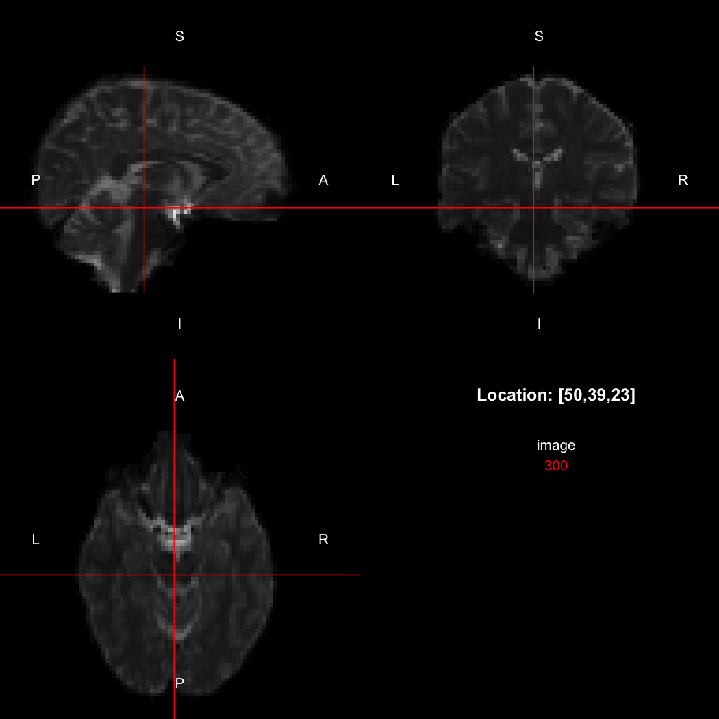
We can also use the RNifti image viewer to visualise the
image.
view(image)
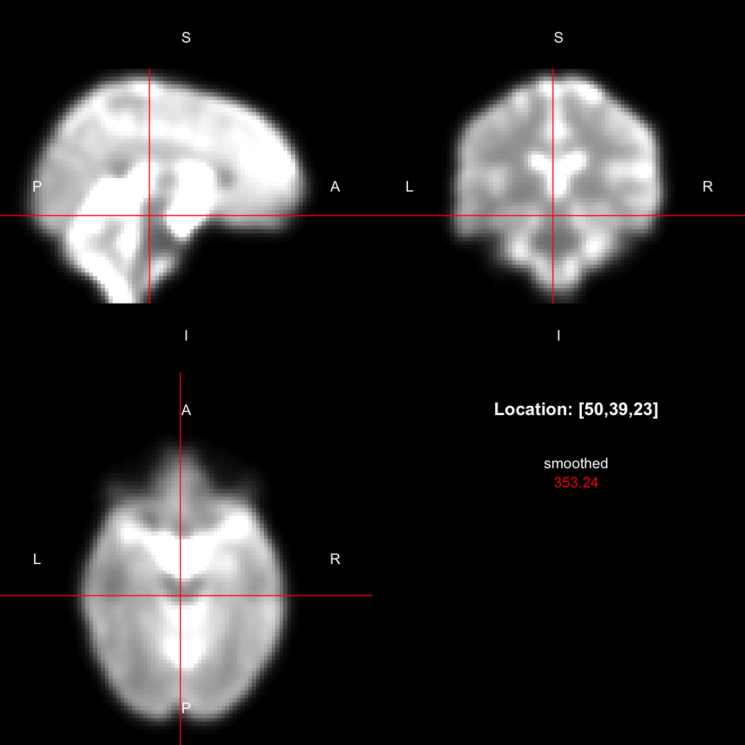
A simple example operation would be to smooth the image with a Gaussian smoothing kernel of standard deviation 4 mm. We can use standard R syntax to perform this operation, return a result, and then show it:
smoothed <- run(smooth_gauss(image, 4))
view(smoothed)
## Setting window to (0, 549.9)
Here, smooth_gauss() requests the smoothing operation,
and run() actually runs the pipeline and returns the
processed image.
However, the pipe syntax provides an alternative, which can be
further simplified because calling view() on a pipeline
will implicitly run it.
image %>% smooth_gauss(4) %>% view()
## Setting window to (0, 549.9)
Notice now smooth_gauss() is now called with only one
argument, and view() with none, because the input to the
pipe (%>%) is implicitly added first. The benefits to
readability of this approach increase substantially as more operations
are added to the chain:
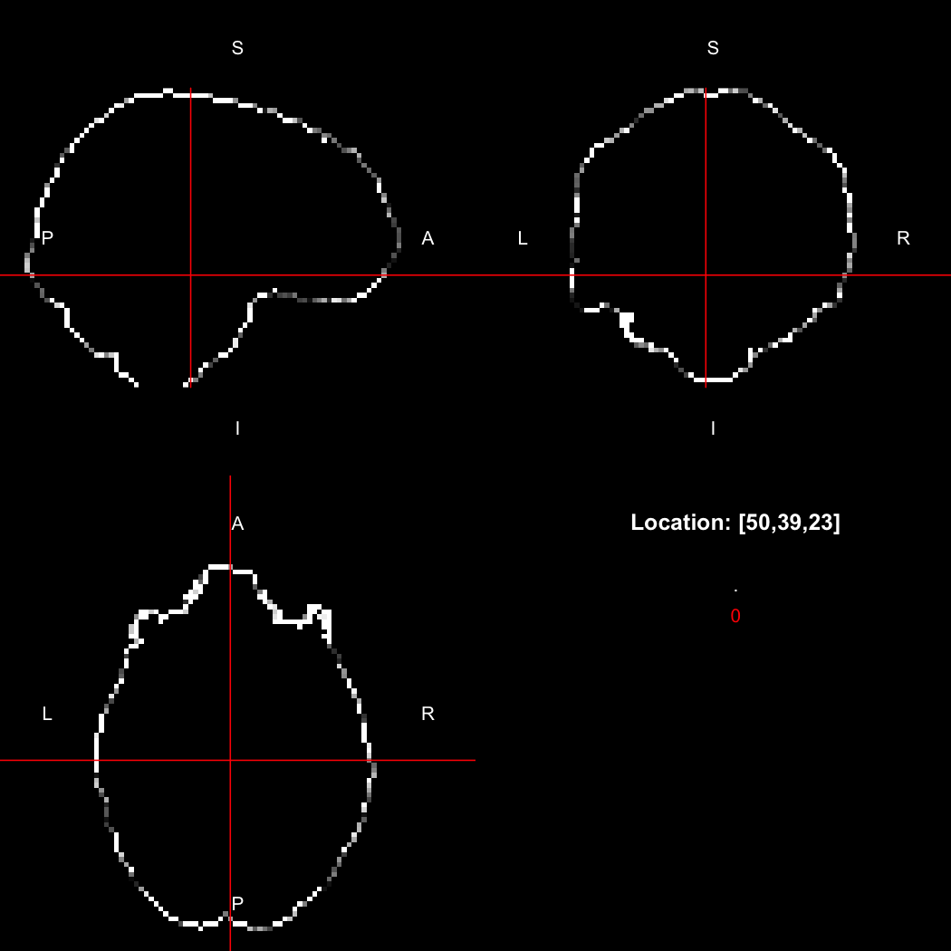
image %>% kernel_sphere(radius=3) %>% dilate() %>% subtract(image) %>% view()
## Setting window to (0, 60)
This example sets up a spherical kernel of radius 3 mm, dilates the image with it, and then subtracts the original image from the result to leave just the outer edge of the imaged object.
These binaries (installable software) and packages are in development.
They may not be fully stable and should be used with caution. We make no claims about them.
Health stats visible at Monitor.