The hardware and bandwidth for this mirror is donated by dogado GmbH, the Webhosting and Full Service-Cloud Provider. Check out our Wordpress Tutorial.
If you wish to report a bug, or if you are interested in having us mirror your free-software or open-source project, please feel free to contact us at mirror[@]dogado.de.
The goal of ibdfindr is to detect genomic regions shared identical by descent (IBD) between two individuals, using SNP genotypes. It does so by fitting a continuous-time hidden Markov model (HMM) to the data.
Until ibdfindr becomes available on CRAN, you may install the development version from GitHub:
remotes::install_github("magnusdv/ibdfindr")library(ibdfindr)As an example we consider the built-in dataset
cousinsDemo, which contains almost 4000 SNP genotypes for
two related individuals (in fact, a pair of cousins).
head(cousinsDemo)#> CHROM MARKER MB CM A1 A2 FREQ1 ID1 ID2
#> 1 1 rs9442372 1.083324 0.0000000 A G 0.3890 A/G G/G
#> 2 1 rs4648727 1.844830 0.1803812 A C 0.3628 A/C A/C
#> 3 1 rs10910082 2.487496 1.2670505 C T 0.3740 C/T C/T
#> 4 1 rs6695131 3.084360 1.9782286 C T 0.5719 C/T C/T
#> 5 1 rs3765703 3.675872 4.8403127 G T 0.4058 G/G T/T
#> 6 1 rs7367066 3.887191 5.7748481 C T 0.6739 C/C C/CThe function findIBD() conveniently wraps the key steps
of the package:
fitHMM())findSegments())ibdPosteriors())ibd = findIBD(cousinsDemo)
#> Individuals: ID1, ID2
#> Chromosome type: autosomal
#> Fitting HMM parameters...
#> Optimising `k1` and `a` jointly; method: L-BFGS-B
#> k1 = 0.185, a = 7.430
#> Finding IBD segments...
#> 14 segments (total length: 597.21 cM)
#> Calculating IBD posteriors...
#> Analysis complete in 0.937 secsFor details of the different steps, see the documentation of the
individual functions: fitHMM(),
findSegments(), and ibdPosteriors().
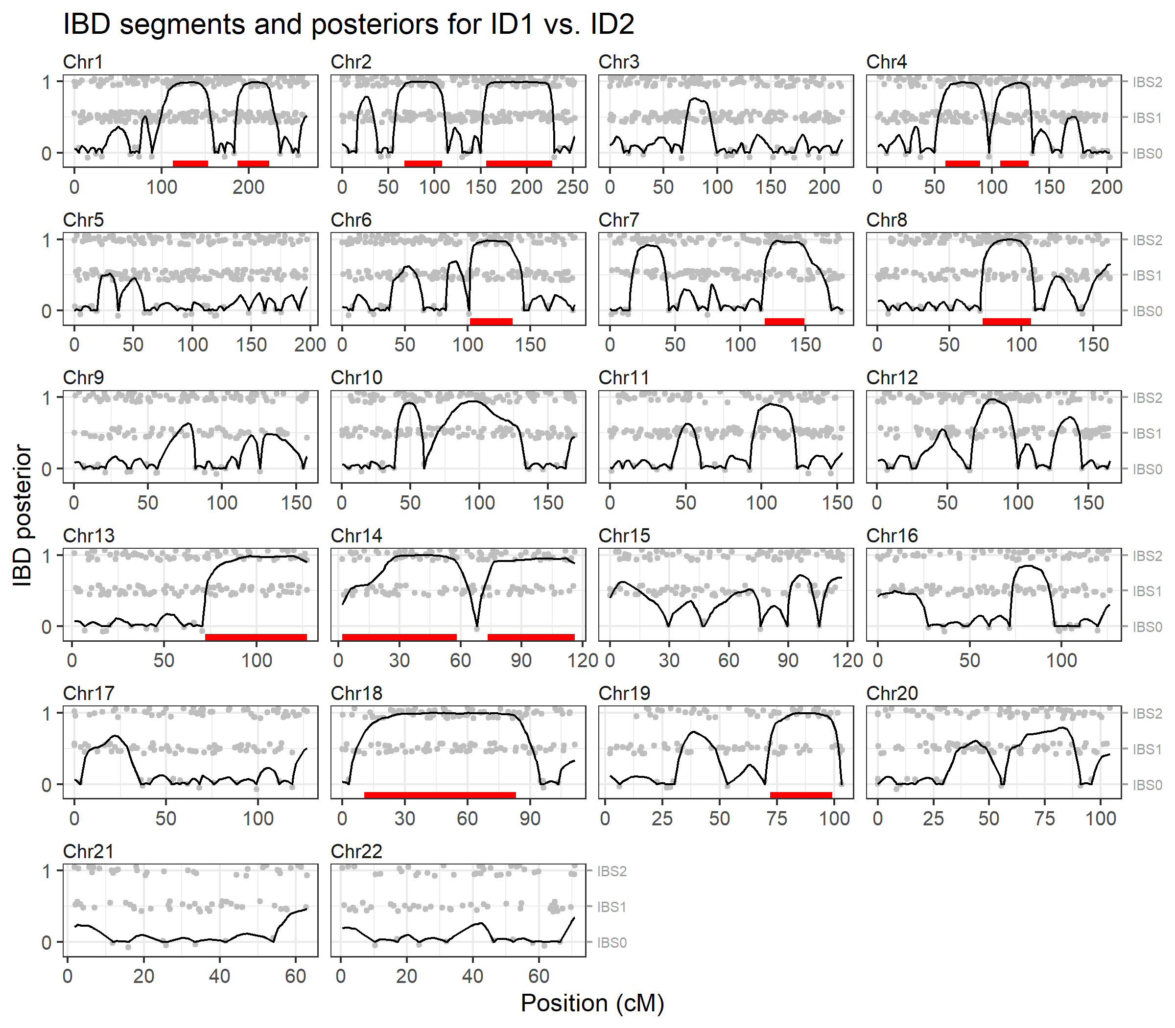
To visualise the results we pass the output to
plotIBD(). This plots the posterior probabilities on a
background (grey points) showing the identity-by-state (IBS) status at
each marker, i.e. whether the individuals have 0, 1 or 2 alleles in
common. Inferred IBD regions are shown as red segments at the bottom of
each chromosome panel.
plotIBD(ibd)
We may also inspect the identified segments as a data frame, showing the start and end positions, and the number of markers in each segment:
ibd$segments
#>    chrom    startCM     endCM   n
#> 1      1 113.000492 153.08623  54
#> 2      1 186.630319 223.39542  46
#> 3      2  67.118524 108.35905  50
#> 4      2 156.120361 227.62362  90
#> 5      4  59.474215  89.85522  41
#> 6      4 106.931772 131.69280  35
#> 7      6 102.041153 136.17734  43
#> 8      7 118.702115 149.11283  38
#> 9      8  72.976430 106.82971  55
#> 10    13  72.049460 127.22724  63
#> 11    14   1.808552  58.07117  67
#> 12    14  73.201009 116.00254  49
#> 13    18  10.592411  83.28443 101
#> 14 19 72.014020 99.15558 34The brothersX dataset contains genotypes for two
brothers typed with 246 X-chromosomal SNPs. The analysis below indicates
that they share 3 IBD segments on the X chromosome.
ibdX = findIBD(brothersX)
#> Individuals: ID1, ID2
#> Chromosome type: X (male/male)
#> Fitting HMM parameters...
#>   Optimising `k1` and `a` jointly; method: L-BFGS-B
#>   k1 = 0.649, a = 6.635
#> Finding IBD segments...
#>   3 segments (total length: 88.05 cM)
#> Calculating IBD posteriors...
#> Analysis complete in 0.1 secs

plotIBD(ibdX)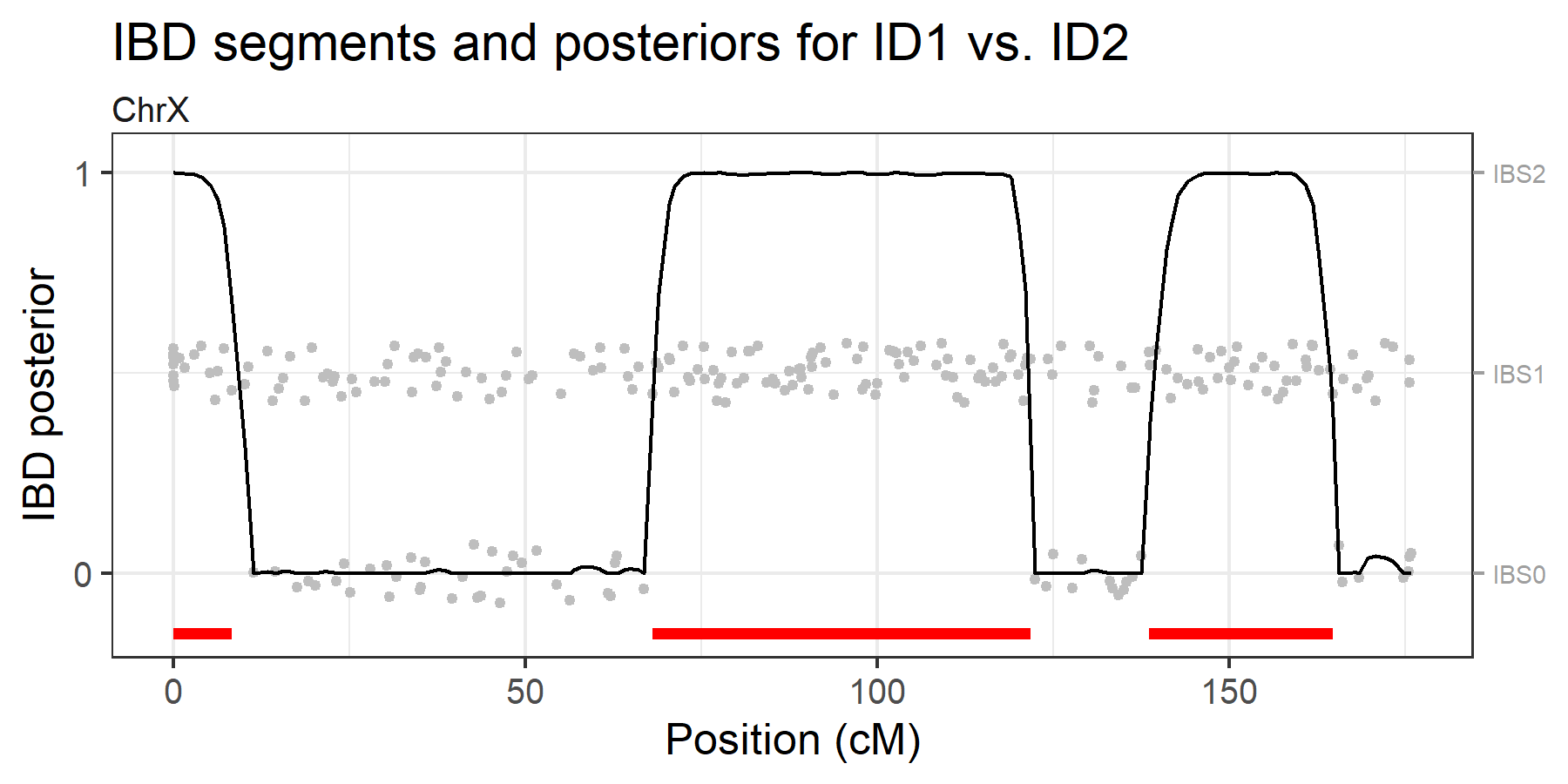
These binaries (installable software) and packages are in development.
They may not be fully stable and should be used with caution. We make no claims about them.
Health stats visible at Monitor.