
The hardware and bandwidth for this mirror is donated by dogado GmbH, the Webhosting and Full Service-Cloud Provider. Check out our Wordpress Tutorial.
If you wish to report a bug, or if you are interested in having us mirror your free-software or open-source project, please feel free to contact us at mirror[@]dogado.de.

hts is retired, with minimum maintenance to keep it on CRAN. We recommend using the fable package instead.
The R package hts presents functions to create, plot and forecast hierarchical and grouped time series.
You can install the stable version on R CRAN.
install.packages('hts', dependencies = TRUE)You can also install the development version from Github
# install.packages("devtools")
devtools::install_github("earowang/hts")library(hts)
#> Loading required package: forecast
#> Registered S3 method overwritten by 'quantmod':
#> method from
#> as.zoo.data.frame zoo
# hts example 1
print(htseg1)
#> Hierarchical Time Series
#> 3 Levels
#> Number of nodes at each level: 1 2 5
#> Total number of series: 8
#> Number of observations per series: 10
#> Top level series:
#> Time Series:
#> Start = 1992
#> End = 2001
#> Frequency = 1
#> [1] 48.74808 49.48047 49.93238 50.24070 50.60846 50.84851 51.70922 51.94330
#> [9] 52.57796 53.21496
summary(htseg1)
#> Hierarchical Time Series
#> 3 Levels
#> Number of nodes at each level: 1 2 5
#> Total number of series: 8
#> Number of observations per series: 10
#> Top level series:
#> Time Series:
#> Start = 1992
#> End = 2001
#> Frequency = 1
#> [1] 48.74808 49.48047 49.93238 50.24070 50.60846 50.84851 51.70922 51.94330
#> [9] 52.57796 53.21496
#>
#> Labels:
#> [1] "Level 0" "Level 1" "Level 2"
aggts1 <- aggts(htseg1)
aggts2 <- aggts(htseg1, levels = 1)
aggts3 <- aggts(htseg1, levels = c(0, 2))
plot(htseg1, levels = 1)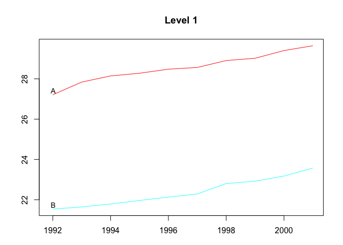
smatrix(htseg1)  # Return the dense mode
#>      [,1] [,2] [,3] [,4] [,5]
#> [1,]    1    1    1    1    1
#> [2,]    1    1    1    0    0
#> [3,]    0    0    0    1    1
#> [4,]    1    0    0    0    0
#> [5,]    0    1    0    0    0
#> [6,]    0    0    1    0    0
#> [7,]    0    0    0    1    0
#> [8,]    0    0    0    0    1

# Forecasts
fcasts1.bu <- forecast(
  htseg1, h = 4, method = "bu", fmethod = "ets", parallel = TRUE
)
aggts4 <- aggts(fcasts1.bu)
summary(fcasts1.bu)
#> Hierarchical Time Series
#> 3 Levels
#> Number of nodes at each level: 1 2 5
#> Total number of series: 8
#> Number of observations in each historical series: 10
#> Number of forecasts per series: 4
#> Top level series of forecasts:
#> Time Series:
#> Start = 2002
#> End = 2005
#> Frequency = 1
#> [1] 53.2149 53.2149 53.2149 53.2149
#>
#> Method: Bottom-up forecasts
#> Forecast method: ETS
fcasts1.td <- forecast(
  htseg1, h = 4, method = "tdfp", fmethod = "arima", keep.fitted = TRUE
)
summary(fcasts1.td)  # When keep.fitted = TRUE, return in-sample accuracy
#> Hierarchical Time Series
#> 3 Levels
#> Number of nodes at each level: 1 2 5
#> Total number of series: 8
#> Number of observations in each historical series: 10
#> Number of forecasts per series: 4
#> Top level series of forecasts:
#> Time Series:
#> Start = 2002
#> End = 2005
#> Frequency = 1
#> [1] 53.71128 54.20760 54.70392 55.20024
#>
#> Method: Top-down forecasts using forecasts proportions
#> Forecast method: Arima
#> In-sample error measures at the bottom level:
#>                AA           AB          AC          BA           BB
#> ME   0.0007719336 0.0009183738 0.001003812 0.001043247  0.001087807
#> RMSE 0.1298400018 0.0515879830 0.040306867 0.037462277  0.105015065
#> MAE  0.0978321731 0.0436089571 0.033210387 0.027003846  0.081906948
#> MAPE 1.1275970221 0.4534439625 0.323535559 0.251066115  0.691364891
#> MPE  0.0367879336 0.0069220593 0.006785872 0.007787895 -0.011087494
#> MASE 0.6825678136 0.5197483057 0.774250880 0.447950006  0.493684443
fcasts1.comb <- forecast(
  htseg1, h = 4, method = "comb", fmethod = "ets", keep.fitted = TRUE
)
aggts4 <- aggts(fcasts1.comb)
plot(fcasts1.comb, levels = 2)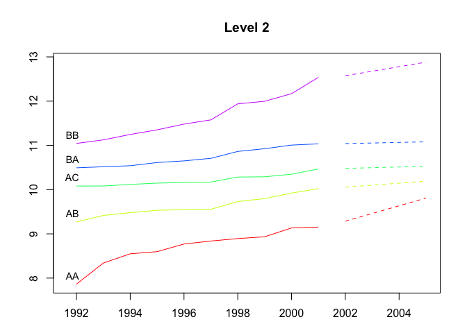
plot(fcasts1.comb, include = 5, levels = c(1, 2))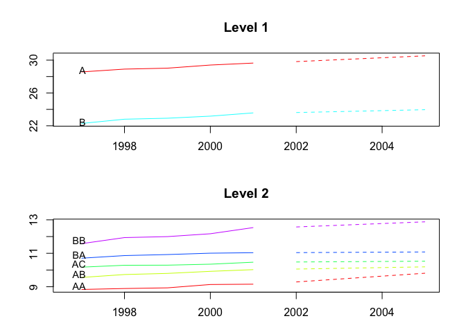
# hts example 2
data <- window(htseg2, start = 1992, end = 2002)
test <- window(htseg2, start = 2003)
fcasts2.mo <- forecast(
  data, h = 5, method = "mo", fmethod = "ets", level = 1,
  keep.fitted = TRUE, keep.resid = TRUE
)
accuracy.gts(fcasts2.mo, test)
#>           Total          A          B        A10          A20         B30
#> ME   -0.1463168 -0.2229191 0.07660233 -0.2283919  0.005472780 -0.01989880
#> RMSE  0.1500119  0.2452066 0.14257606  0.2523329  0.009805797  0.02928379
#> MAE   0.1463168  0.2229191 0.11693106  0.2283919  0.009268225  0.02409282
#> MAPE  9.3179712  7.5314777 2.36244104  8.7993966  2.460560011  1.71428541
#> MPE  -9.3179712  7.5314777 1.45433283  8.7993966 -1.631079601 -1.39920296
#> MASE  0.4617075  1.2506962 0.84324674  1.5148807  0.337389275  0.52860991
#>             B40        A10A       A10B          A10C         A20A         A20B
#> ME   0.09650113 -0.05448806 -0.1733829 -0.0005209908  0.007965591 -0.002492811
#> RMSE 0.17060895  0.06809235  0.1867174  0.0100661166  0.012682474  0.008654148
#> MAE  0.14102388  0.05448806  0.1733829  0.0088897199  0.010413971  0.007052515
#> MAPE 3.98260313  4.37476593 21.6158413  1.5612291069  3.334410408 13.402921842
#> MPE  2.54768302  4.37476593 21.6158413  0.0605205225 -2.607467068 -2.981389244
#> MASE 1.51492018  0.51577051  5.3650162  0.6942763126  0.820393749  0.477277465
#>            B30A        B30B        B30C        B40A      B40B
#> ME   0.01212900 -0.01099794 -0.02102986 -0.04273559 0.1392367
#> RMSE 0.01311771  0.01422607  0.02442915  0.06656885 0.2344656
#> MAE  0.01212900  0.01099794  0.02102986  0.04273559 0.1811449
#> MAPE 4.13200908  2.39939647  3.26532975  3.09570196 8.2253477
#> MPE  4.13200908 -2.39939647 -3.26532975 -3.09570196 5.9207223
#> MASE 0.49670326  1.22312029  1.72843722  0.82335272 4.3982548
accuracy.gts(fcasts2.mo, test, levels = 1)
#>               A          B
#> ME   -0.2229191 0.07660233
#> RMSE  0.2452066 0.14257606
#> MAE   0.2229191 0.11693106
#> MAPE  7.5314777 2.36244104
#> MPE   7.5314777 1.45433283
#> MASE  1.2506962 0.84324674
fcasts2.td <- forecast(
  data, h = 5, method = "tdgsa", fmethod = "ets",
  keep.fitted = TRUE, keep.resid = TRUE
)
plot(fcasts2.td, include = 5)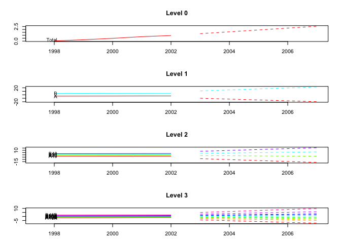
plot(fcasts2.td, include = 5, levels = c(0, 2))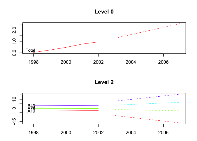
# gts example
plot(infantgts, levels = 1)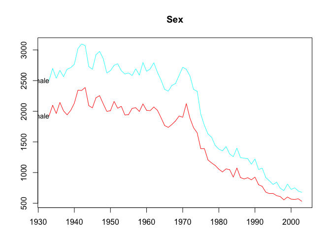
fcasts3.comb <- forecast(infantgts, h = 4, method = "comb", fmethod = "ets")
agg_gts1 <- aggts(fcasts3.comb, levels = 1)
agg_gts2 <- aggts(fcasts3.comb, levels = 1, forecasts = FALSE)
plot(fcasts3.comb)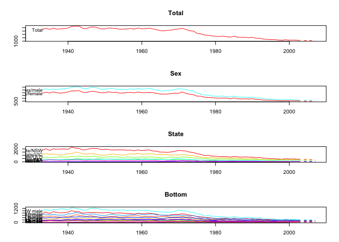
plot(fcasts3.comb, include = 5, levels = c(1, 2))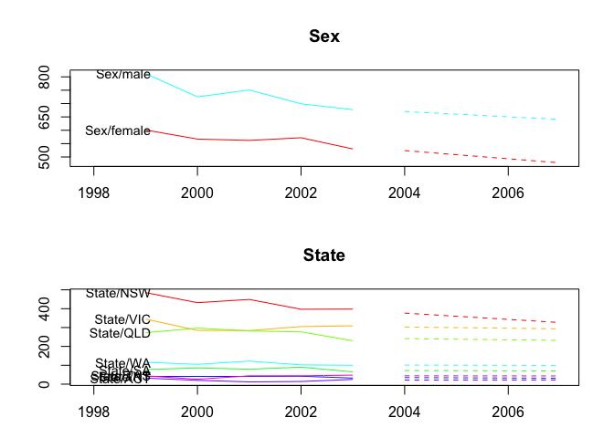
fcasts3.combsd <- forecast(
  infantgts, h = 4, method = "comb", fmethod = "ets",
  weights = "sd", keep.fitted = TRUE
)

fcasts3.combn <- forecast(
  infantgts, h = 4, method = "comb", fmethod = "ets",
  weights = "nseries", keep.resid = TRUE
)This package is free and open source software, licensed under GPL (>= 2).
These binaries (installable software) and packages are in development.
They may not be fully stable and should be used with caution. We make no claims about them.
Health stats visible at Monitor.