The hardware and bandwidth for this mirror is donated by dogado GmbH, the Webhosting and Full Service-Cloud Provider. Check out our Wordpress Tutorial.
If you wish to report a bug, or if you are interested in having us mirror your free-software or open-source project, please feel free to contact us at mirror[@]dogado.de.

healthyR.ts

The Time Series Modeling Companion to healthyR

To view the full wiki, click here: Full healthyR.ts Wiki

healthyR.ts is a comprehensive R package designed specifically for time series analysis and forecasting of hospital administrative and clinical data. Built on the powerful tidymodels ecosystem, it provides a consistent, user-friendly framework that simplifies complex time series workflows.

Why healthyR.ts?

Hospital data analysis often requires handling time series for metrics like: - Average Length of Stay (ALOS) - Readmission rates - Patient volumes and admissions - Bed occupancy rates - Clinical outcomes over time

healthyR.ts takes the guesswork out of time series analysis by providing:

✅ Automated Workflows - One-function solutions for complete modeling pipelines
✅ Visual Analytics - Rich plotting functions for data exploration
✅ Data Generators - Simulate realistic time series for testing and validation
✅ Statistical Tools - Comprehensive suite of time series statistics
✅ Clustering - Feature-based time series clustering capabilities
✅ Forecasting - 15 automated model workflows (ARIMA, Prophet, XGBoost, and more)

Key Features

🤖 Automatic Modeling Workflows

Complete end-to-end modeling pipelines in a single function call:

ts_auto_arima() - Automatic ARIMA modeling
ts_auto_prophet_reg() - Facebook’s Prophet algorithm
ts_auto_xgboost() - Gradient boosting for time series
ts_auto_nnetar() - Neural network autoregression
Plus 11 more specialized workflows!

Each function handles recipe creation, model specification, workflow setup, model fitting, tuning, and calibration automatically.

📊 Visualization Suite

Calendar heatmaps for temporal patterns
Time series clustering plots
Velocity, acceleration, and growth visualizations
QQ plots and scedasticity analysis
Moving average and SMA plots
Event analysis visualizations

🎲 Data Generation

Generate synthetic time series data for testing: - Random walks and Brownian motion - Geometric Brownian motion - ARIMA simulations - Custom parameter configurations

📈 Statistical Analysis

ADF stationarity tests
Fast Fourier Transform (FFT) analysis
Confidence intervals
Lag correlation analysis
Time series feature extraction

Installation

Stable Release (CRAN)

Install the latest stable version from CRAN:

install.packages("healthyR.ts")

Development Version

Get the latest features and bug fixes from GitHub:

# install.packages("devtools")
devtools::install_github("spsanderson/healthyR.ts")

Quick Start

Basic Example: Random Walk Simulation

Generate and visualize random walk data to understand market volatility or patient flow variations:

library(healthyR.ts)
library(ggplot2)

df <- ts_random_walk()

head(df)
#> # A tibble: 6 × 4
#>     run     x       y cum_y
#>   <dbl> <dbl>   <dbl> <dbl>
#> 1     1     1  0.113  1113.
#> 2     1     2  0.119  1245.
#> 3     1     3 -0.0178 1223.
#> 4     1     4  0.141  1396.
#> 5     1     5 -0.163  1169.
#> 6     1     6 -0.0485 1112.

Now that the data has been generated, lets take a look at it.

df %>%
   ggplot(
       mapping = aes(
           x = x
           , y = cum_y
           , color = factor(run)
           , group = factor(run)
        )
    ) +
    geom_line(alpha = 0.8) +
    ts_random_walk_ggplot_layers(df)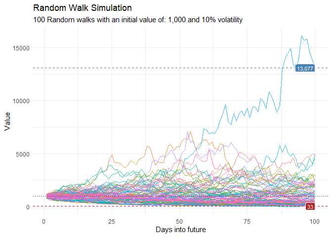

That is still pretty noisy, so lets see this in a different way. Lets clear this up a bit to make it easier to see the full range of the possible volatility of the random walks.

library(dplyr)
library(ggplot2)

df %>%
    group_by(x) %>%
    summarise(
        min_y = min(cum_y),
        max_y = max(cum_y)
    ) %>%
    ggplot(
        aes(x = x)
    ) +
    geom_line(aes(y = max_y), color = "steelblue") +
    geom_line(aes(y = min_y), color = "firebrick") +
    geom_ribbon(aes(ymin = min_y, ymax = max_y), alpha = 0.2) +
    ts_random_walk_ggplot_layers(df)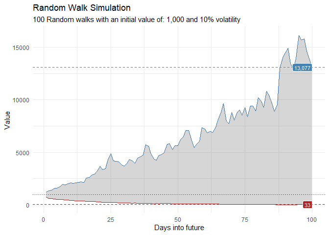

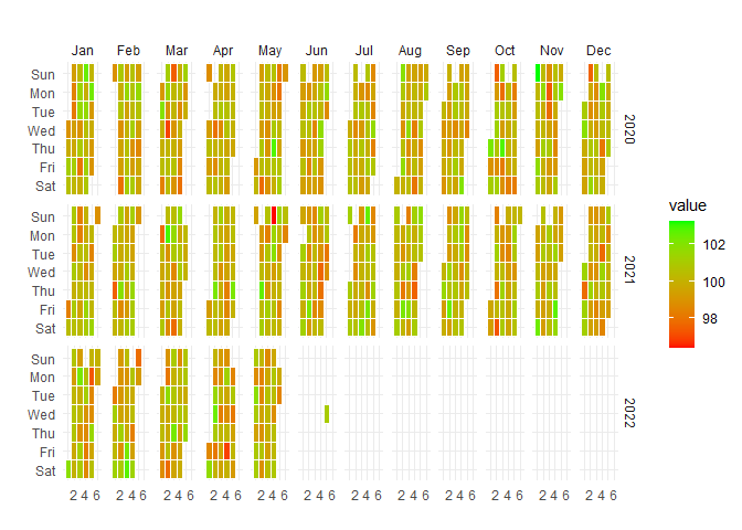
Calendar Heatmap Visualization

Visualize temporal patterns in your data with calendar heatmaps - perfect for identifying seasonal trends or unusual patterns in hospital metrics:

data_tbl <- data.frame(
  date_col = seq.Date(
    from = as.Date("2020-01-01"),
    to   = as.Date("2022-06-01"),
    length.out = 365*2 + 180
    ),
  value = rnorm(365*2+180, mean = 100)
)

ts_calendar_heatmap_plot(
  .data          = data_tbl
  , .date_col    = date_col
  , .value_col   = value
  , .interactive = FALSE
)

Time Series Clustering

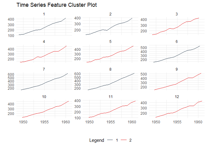
Discover patterns by clustering time series based on their statistical features:

data_tbl <- ts_to_tbl(AirPassengers) %>%
  mutate(group_id = rep(1:12, 12))

output <- ts_feature_cluster(
  .data = data_tbl,
  .date_col = date_col,
  .value_col = value,
  group_id,
  .features = c("acf_features","entropy"),
  .scale = TRUE,
  .prefix = "ts_",
  .centers = 3
)

ts_feature_cluster_plot(
  .data = output,
  .date_col = date_col,
  .value_col = value,
  .center = 2,
  group_id
)

#> $plot
#> $plot$static_plot

#> 
#> $plot$plotly_plot
#> 
#> 
#> $data
#> $data$original_data
#> # A tibble: 144 × 4
#>    index     date_col   value group_id
#>    <yearmon> <date>     <dbl>    <int>
#>  1 Jan 1949  1949-01-01   112        1
#>  2 Feb 1949  1949-02-01   118        2
#>  3 Mar 1949  1949-03-01   132        3
#>  4 Apr 1949  1949-04-01   129        4
#>  5 May 1949  1949-05-01   121        5
#>  6 Jun 1949  1949-06-01   135        6
#>  7 Jul 1949  1949-07-01   148        7
#>  8 Aug 1949  1949-08-01   148        8
#>  9 Sep 1949  1949-09-01   136        9
#> 10 Oct 1949  1949-10-01   119       10
#> # ℹ 134 more rows
#> 
#> $data$kmm_data_tbl
#> # A tibble: 3 × 3
#>   centers k_means  glance          
#>     <int> <list>   <list>          
#> 1       1 <kmeans> <tibble [1 × 4]>
#> 2       2 <kmeans> <tibble [1 × 4]>
#> 3       3 <kmeans> <tibble [1 × 4]>
#> 
#> $data$user_item_tbl
#> # A tibble: 12 × 8
#>    group_id ts_x_acf1 ts_x_acf10 ts_diff1_acf1 ts_diff1_acf10 ts_diff2_acf1
#>       <int>     <dbl>      <dbl>         <dbl>          <dbl>         <dbl>
#>  1        1     0.741       1.55       -0.0995          0.474       -0.182 
#>  2        2     0.730       1.50       -0.0155          0.654       -0.147 
#>  3        3     0.766       1.62       -0.471           0.562       -0.620 
#>  4        4     0.715       1.46       -0.253           0.457       -0.555 
#>  5        5     0.730       1.48       -0.372           0.417       -0.649 
#>  6        6     0.751       1.61        0.122           0.646        0.0506
#>  7        7     0.745       1.58        0.260           0.236       -0.303 
#>  8        8     0.761       1.60        0.319           0.419       -0.319 
#>  9        9     0.747       1.59       -0.235           0.191       -0.650 
#> 10       10     0.732       1.50       -0.0371          0.269       -0.510 
#> 11       11     0.746       1.54       -0.310           0.357       -0.556 
#> 12       12     0.735       1.51       -0.360           0.294       -0.601 
#> # ℹ 2 more variables: ts_seas_acf1 <dbl>, ts_entropy <dbl>
#> 
#> $data$cluster_tbl
#> # A tibble: 12 × 9
#>    cluster group_id ts_x_acf1 ts_x_acf10 ts_diff1_acf1 ts_diff1_acf10
#>      <int>    <int>     <dbl>      <dbl>         <dbl>          <dbl>
#>  1       2        1     0.741       1.55       -0.0995          0.474
#>  2       2        2     0.730       1.50       -0.0155          0.654
#>  3       1        3     0.766       1.62       -0.471           0.562
#>  4       1        4     0.715       1.46       -0.253           0.457
#>  5       1        5     0.730       1.48       -0.372           0.417
#>  6       2        6     0.751       1.61        0.122           0.646
#>  7       2        7     0.745       1.58        0.260           0.236
#>  8       2        8     0.761       1.60        0.319           0.419
#>  9       1        9     0.747       1.59       -0.235           0.191
#> 10       1       10     0.732       1.50       -0.0371          0.269
#> 11       1       11     0.746       1.54       -0.310           0.357
#> 12       1       12     0.735       1.51       -0.360           0.294
#> # ℹ 3 more variables: ts_diff2_acf1 <dbl>, ts_seas_acf1 <dbl>, ts_entropy <dbl>
#> 
#> 
#> $kmeans_object
#> $kmeans_object[[1]]
#> K-means clustering with 2 clusters of sizes 7, 5
#> 
#> Cluster means:
#>   ts_x_acf1 ts_x_acf10 ts_diff1_acf1 ts_diff1_acf10 ts_diff2_acf1 ts_seas_acf1
#> 1 0.7387865   1.528308    -0.2909349      0.3638392    -0.5916245    0.2930543
#> 2 0.7456468   1.568532     0.1172685      0.4858013    -0.1799728    0.2876449
#>   ts_entropy
#> 1  0.6438176
#> 2  0.4918321
#> 
#> Clustering vector:
#>  [1] 2 2 1 1 1 2 2 2 1 1 1 1
#> 
#> Within cluster sum of squares by cluster:
#> [1] 0.3660630 0.3704304
#>  (between_SS / total_SS =  59.8 %)
#> 
#> Available components:
#> 
#> [1] "cluster"      "centers"      "totss"        "withinss"     "tot.withinss"
#> [6] "betweenss"    "size"         "iter"         "ifault"

Event Analysis

Analyze time series behavior before and after significant events (e.g., policy changes, new treatments):

library(dplyr)
df <- ts_to_tbl(AirPassengers) %>% select(-index)

ts_time_event_analysis_tbl(
  .data = df,
  .horizon = 6,
  .date_col = date_col,
  .value_col = value,
  .direction = "both"
) %>%
  ts_event_analysis_plot()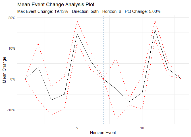



ts_time_event_analysis_tbl(
  .data = df,
  .horizon = 6,
  .date_col = date_col,
  .value_col = value,
  .direction = "both"
) %>%
  ts_event_analysis_plot(.plot_type = "individual")

ARIMA Simulation

Generate realistic ARIMA time series for testing and validation:

output <- ts_arima_simulator()
output$plots$static_plot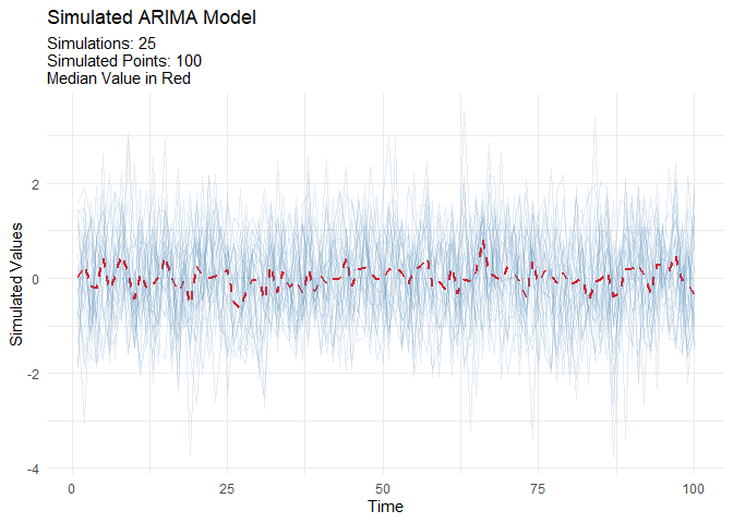

Available Models

Automated Workflow Functions

Each function creates a complete modeling pipeline including recipe, model specification, workflow, fitting, and calibration:

Function	Model Type	Description
`ts_auto_arima()`	ARIMA	Automatic ARIMA with auto-tuning
`ts_auto_arima_xgboost()`	Hybrid	ARIMA errors with XGBoost
`ts_auto_prophet_reg()`	Prophet	Facebook’s Prophet algorithm
`ts_auto_prophet_boost()`	Hybrid	Prophet with XGBoost
`ts_auto_xgboost()`	ML	Gradient boosting
`ts_auto_nnetar()`	Neural Net	Neural network autoregression
`ts_auto_exp_smoothing()`	ETS	Exponential smoothing
`ts_auto_smooth_es()`	Smooth	Smooth package ETS
`ts_auto_theta()`	Theta	Theta method
`ts_auto_croston()`	Croston	For intermittent demand
`ts_auto_lm()`	Linear	Linear regression with time features
`ts_auto_mars()`	MARS	Multivariate adaptive regression splines
`ts_auto_glmnet()`	GLM	Elastic net regression
`ts_auto_svm_poly()`	SVM	Support vector machine (polynomial)
`ts_auto_svm_rbf()`	SVM	Support vector machine (radial)

Function Categories

healthyR.ts includes 90+ functions organized into these categories:

📊 Data Generators: Create synthetic time series data (random walks, Brownian motion, ARIMA)
📈 Plotting Functions: Comprehensive visualization suite for time series
🔍 Clustering: Feature-based time series clustering and analysis
🤖 Forecasting: Automated modeling workflows and model comparison
📐 Statistical Functions: Tests, transformations, and time series statistics
🔧 Utilities: Helper functions for data manipulation and transformation
📉 Augment Functions: Add features like velocity, acceleration, and growth rates
🧮 Vector Functions: Vectorized operations for time series
🔬 Recipe Steps: Custom tidymodels recipe steps for time series

Documentation

📘 Getting Started Vignette - Comprehensive introduction
📗 Function Reference - Complete function documentation
📙 Package Website - Full documentation site
📕 News/Changelog - Version history and updates

Learning Resources

Vignettes

Example Use Cases

Hospital Admissions Forecasting - Predict daily/weekly admissions using multiple models
Length of Stay Analysis - Analyze and forecast ALOS trends
Readmission Rate Monitoring - Track and predict readmission patterns
Resource Planning - Forecast bed occupancy and staffing needs
Seasonal Pattern Detection - Identify and visualize seasonal trends in clinical data

Contributing

Contributions are welcome! Here’s how you can help:

🐛 Report bugs via GitHub Issues
💡 Suggest features through issue requests
🔧 Submit pull requests for bug fixes or new features
📖 Improve documentation by suggesting clarifications or additions

Please follow the tidyverse style guide for code contributions.

healthyR - Hospital data analysis companion package
healthyR.ai - Machine learning companion for healthcare
healthyverse - Meta-package loading all healthyR packages

Citation

If you use healthyR.ts in your research or publications, please cite:

citation("healthyR.ts")

Support

📧 Email: spsanderson@gmail.com
🐦 Issues: GitHub Issue Tracker
🌐 Website: https://www.spsanderson.com/healthyR.ts/

These binaries (installable software) and packages are in development.
They may not be fully stable and should be used with caution. We make no claims about them.
Health stats visible at Monitor.