The hardware and bandwidth for this mirror is donated by dogado GmbH, the Webhosting and Full Service-Cloud Provider. Check out our Wordpress Tutorial.
If you wish to report a bug, or if you are interested in having us mirror your free-software or open-source project, please feel free to contact us at mirror[@]dogado.de.

hcinfer

hcinfer computes heteroskedasticity-consistent covariance estimators and normal Wald inference for ordinary least squares models. The currently implemented covariance matrix estimators are listed below.

Implemented Estimators

The table below is generated by hc_methods() and lists the covariance matrix estimators currently implemented in hcinfer.

type	label	description	default_arguments
hc0	HC0	White heteroskedasticity-consistent estimator.	none
hc1	HC1	HC0 with degrees-of-freedom scaling.	none
hc2	HC2	Leverage-adjusted estimator with exponent 1.	none
hc3	HC3	Leverage-adjusted estimator with exponent 2.	none
hc4	HC4	Adaptive leverage correction by Cribari-Neto.	none
hc4m	HC4m	Modified HC4 correction by Cribari-Neto and da Silva.	none
hc5	HC5	High-leverage correction by Cribari-Neto, Souza, and Vasconcellos.	k = 0.7
hc5m	HC5m	Modified HC5 correction by Li, Zhang, Zhang, and Wang.	k = 0.7, k1 = 1, k2 = 0, k3 = 1, gamma1 = 1, gamma2 = 1.5
hcbeta	HCbeta	Beta-distribution leverage correction.	c1 = 7, c2 = 0.75, lower = 0.01, upper = 0.99

Installation

# install.packages("hcinfer")

# Development version
remotes::install_github("prdm0/hcinfer")

Basic Use

library(hcinfer)

schools <- PublicSchools
schools$income_scaled <- schools$income / 10000
schools$income_scaled_sq <- schools$income_scaled^2

fit <- lm(expenditure ~ income_scaled + income_scaled_sq, data = schools)

result <- hcinfer(fit)

The default estimator is HCbeta. Use tests() and confint() to extract the main inferential quantities as tibbles.

tests(result)
#> # A tibble: 3 × 8
#>   term             estimate null_value std_error z_value p_value alpha reject
#>   <chr>               <dbl>      <dbl>     <dbl>   <dbl>   <dbl> <dbl> <lgl>
#> 1 (Intercept)          833.          0      851.   0.979   0.328  0.05 FALSE
#> 2 income_scaled      -1834.          0     2309.  -0.794   0.427  0.05 FALSE
#> 3 income_scaled_sq    1587.          0     1547.   1.03    0.305  0.05 FALSE
confint(result)
#> # A tibble: 3 × 4
#>   term             conf_low conf_high level
#>   <chr>               <dbl>     <dbl> <dbl>
#> 1 (Intercept)         -834.     2500.  0.95
#> 2 income_scaled      -6359.     2691.  0.95
#> 3 income_scaled_sq   -1446.     4620.  0.95

Confidence Intervals

The plot() method displays the robust confidence intervals and marks the null value used in the tests.

plot(result)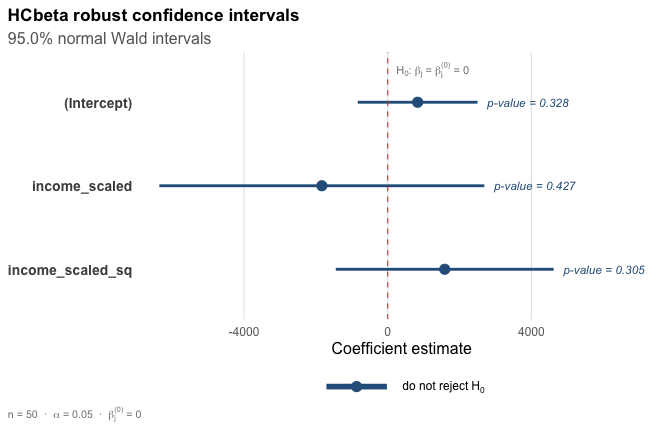

Robust confidence intervals for the public-schools regression coefficients.

Diagnostics

Use vcov_hc() when you only need the robust covariance matrix and its diagnostics. The plot() method for this object shows leverage values and HC adjustment factors.

cov_hcbeta <- vcov_hc(fit)
plot(cov_hcbeta)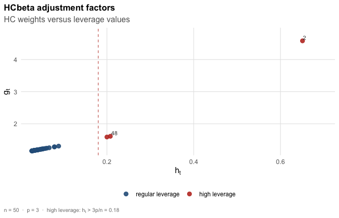

HCbeta adjustment factors plotted against leverage values for the public-schools regression.

Main Functions

hc_methods()
coef(result)
vcov(result)

The most common workflow is:

fit <- lm(y ~ x1 + x2, data = data)
result <- hcinfer(fit, type = "hcbeta")

summary(result)
tests(result)
confint(result)
plot(result)

Learn More

Start with vignette("introduction", package = "hcinfer") for a compact overview of the package API.

References

White, H. (1980). A heteroskedasticity-consistent covariance matrix estimator and a direct test for heteroskedasticity. Econometrica, 48(4), 817-838. doi:10.2307/1912934.
Hinkley, D. V. (1977). Jackknifing in unbalanced situations. Technometrics, 19(3), 285-292. doi:10.1080/00401706.1977.10489550.
Horn, S. D., Horn, R. A., and Duncan, D. B. (1975). Estimating heteroscedastic variances in linear models. Journal of the American Statistical Association, 70(350), 380-385. doi:10.1080/01621459.1975.10479877.
MacKinnon, J. G. and White, H. (1985). Some heteroskedasticity-consistent covariance matrix estimators with improved finite sample properties. Journal of Econometrics, 29(3), 305-325. doi:10.1016/0304-4076(85)90158-7.
Davidson, R. and MacKinnon, J. G. (1993). Estimation and Inference in Econometrics. Oxford University Press.
Cribari-Neto, F. (2004). Asymptotic inference under heteroskedasticity of unknown form. Computational Statistics and Data Analysis, 45(2), 215-233. doi:10.1016/S0167-9473(02)00366-3.
Cribari-Neto, F. and da Silva, W. B. (2011). A new heteroskedasticity-consistent covariance matrix estimator for the linear regression model. AStA Advances in Statistical Analysis, 95(2), 129-146. doi:10.1007/s10182-010-0141-2.
Cribari-Neto, F., Souza, T. C., and Vasconcellos, K. L. P. (2007). Inference under heteroskedasticity and leveraged data. Communications in Statistics - Theory and Methods, 36(10), 1877-1888. doi:10.1080/03610920601126589.
Li, S., Zhang, N., Zhang, X., and Wang, G. (2016). A new heteroskedasticity-consistent covariance matrix estimator and inference under heteroskedasticity. Journal of Statistical Computation and Simulation, 87(1), 198-210. doi:10.1080/00949655.2016.1198906.
Cunha, M. A., Cribari-Neto, F., and Marinho, P. R. D. (manuscript). A beta-based heteroskedasticity-consistent covariance matrix estimator.

These binaries (installable software) and packages are in development.
They may not be fully stable and should be used with caution. We make no claims about them.
Health stats visible at Monitor.