The hardware and bandwidth for this mirror is donated by dogado GmbH, the Webhosting and Full Service-Cloud Provider. Check out our Wordpress Tutorial.
If you wish to report a bug, or if you are interested in having us mirror your free-software or open-source project, please feel free to contact us at mirror[@]dogado.de.

hairline

Clean, predictable figures for medical and data science, built on ‘ggplot2’. One frame for titles, legends, panels and captions, one type scale, colour-vision checked palettes, and print-ready files. The Python package of the same name draws the same figures from the same design tokens, so an R figure and a Python figure in one manuscript match.

install.packages("hairline")

R 4.3 or later with ‘ggplot2’ 4.0 or later. The bundled font, Hairline Sans, needs no installation for PNG, SVG and HTML; for PDF on macOS without XQuartz, run hl_install_font() once.

From data to a result

Most studies need the same few results: a cohort description, a comparison between groups, effects, events over time. hl_study() takes a data frame once, with the role of each column, checks the data, and returns each result as a figure, a table, the key values and a sentence for the text.

library(hairline)

set.seed(1)
cohort <- data.frame(arm = rep(c("Standard care", "Early mobilisation"), each = 40),
                     age = round(rnorm(80, 64, 12)), sex = sample(c("Female", "Male"), 80, TRUE),
                     months = round(rexp(80, 0.05), 1), died = rbinom(80, 1, 0.4))
study <- hl_study(cohort, group = "arm", time = "months", event = "died",
                  units = c(age = "years", months = "months"))

table_one <- hl_describe(study)    # Table 1: median (IQR) and n (%) per group
table_one$table                    # a data frame
age <- hl_compare(study, "age")    # spread rows per group, Wilcoxon rank-sum
age$text                           # "Age (years), median (IQR): ... (Wilcoxon rank-sum, p = ...)."
survival <- hl_survival(study)     # Kaplan-Meier with numbers at risk and the log-rank test
hl_save(survival$figure, "survival")              # survival.pdf and survival.png

Printing a study lists its checks: missing values, duplicate ids, categories that differ only in case, small groups, numeric columns without a unit. Errors stop the analysis; warnings name the fix.

Charts

Each chart is one call with the data and its column names, and returns a ggplot in the hairline frame: hl_bars(), hl_scatter(), hl_timeseries(), hl_spread(), hl_raincloud(), hl_ridgeline(), hl_kaplan_meier(), hl_forest(), hl_dotplot(), hl_funnel(), hl_correlation(), hl_donut(), hl_partition(), hl_sankey(), hl_chord(), hl_arcs(), hl_venn(), hl_prisma() and hl_risk_of_bias().

admissions <- data.frame(diagnosis = c("Sepsis", "Sepsis", "Trauma", "Cardiac", "Cardiac"),
                         sex = c("Female", "Male", "Male", "Female", "Male"))
figure <- hl_bars(admissions, "diagnosis", by = "sex", subtitle = "Admissions, 2025")
hl_save(figure, "admissions", formats = c("pdf", "png", "svg", "html"))

For anything else, theme_hairline() puts the same frame around your own ggplot:

library(ggplot2)
figure <- ggplot(mtcars, aes(wt, mpg)) + geom_point() +
  labs(title = "Fuel use by weight", x = "Weight (1000 lb)", y = "Miles per gallon") +
  theme_hairline()
hl_save(figure, "fuel", size = "single")

Colours

Groups take a palette’s colours in order, so two groups always get the same two colours and a group keeps its colour in every chart. hl_palettes() lists the six palettes, the purpose sets (two groups, greyscale print, risk of bias) and the ramps for amounts; hl_swatches() draws them; hl_use(palette = "calm") changes the default; hl_use(colors = c("Unit B" = "#e79d01")) pins a colour to a name; scale_fill_hairline_c("blues") gives a ramp to your own ggplots. ?hairline_colours has the details.

Files

hl_save() writes PDF, PNG and TIFF (600 dpi by default), SVG (text kept as text) and self-contained interactive HTML with tooltips. Files carry the figure’s title and subtitle as their description, and no timestamps.

Design

• hl_use(brand = "_brand.yml") applies an institution’s colours, fonts and sizes from a brand.yml file; several files layer from institution to document.
• hl_use(colors = c("Unit B" = "#e79d01")) pins a colour to a name across every chart.
• Palettes are checked for colour-vision separation and contrast; hl_check_palette() reports the numbers.
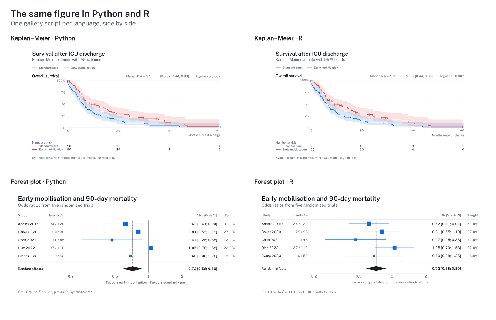
• hl_use(scheme = "dark", accent = "#0b6e4f") draws on a dark surface with an accent for single series.

Gallery

More figures, Python and R side by side, and the colour guide: https://github.com/schradern/hairline.

Author

Nikolas Schrader (hi@nikolasschrader.com), ORCID 0009-0001-4616-3804.

How to cite

If hairline helped you make the figures in your work, please cite it; citation("hairline") prints the reference:

@Manual{schrader2026hairline,
  title = {hairline: Clean, Predictable Figures for Medical and Data Science},
  author = {Nikolas Schrader},
  year = {2026},
  note = {R package version 0.1.0},
  doi = {10.5281/zenodo.23456212},
}

Licence

MIT. The bundled Hairline Sans font is a modified Public Sans (SIL Open Font License 1.1); see inst/COPYRIGHTS.

These binaries (installable software) and packages are in development.
They may not be fully stable and should be used with caution. We make no claims about them.
Health stats visible at Monitor.