
The hardware and bandwidth for this mirror is donated by dogado GmbH, the Webhosting and Full Service-Cloud Provider. Check out our Wordpress Tutorial.
If you wish to report a bug, or if you are interested in having us mirror your free-software or open-source project, please feel free to contact us at mirror[@]dogado.de.
{h3o} is a lightweight R package for interacting with Uber’s H3 Geospatial Indexing
system. The R package uses extendr
to wrap the eponymous h3o Rust
crate, which offers a pure Rust implementation of H3, so no linking
to Uber’s H3 C library. The package is also intended to work with the {sf} package for
geometric operations and as a bonus represents the H3 class as {vctrs}, so they
work seamlessly within a tidyverse workflow.
You can install the release version of {h3o} from CRAN
with:
install.packages("h3o")Or you can install the development version from GitHub with:
# install.packages("pak")
pak::pak("extendr/h3o")H3 vectors can be created from POINT geometry columns
(sfc objects) defined by sf.
library(h3o)
library(dplyr)
library(sf)
library(tibble)

xy <- data.frame(
  x = runif(100, -5, 10),
  y = runif(100, 40, 50)
)

pnts <- st_as_sf(
  xy,
  coords = c("x", "y"),
  crs = 4326
)

pnts |> mutate(h3 = h3_from_points(geometry, 5))
#> Simple feature collection with 100 features and 1 field
#> Geometry type: POINT
#> Dimension:     XY
#> Bounding box:  xmin: -4.906456 ymin: 40.13608 xmax: 9.720642 ymax: 49.77958
#> Geodetic CRS:  WGS 84
#> First 10 features:
#>                       geometry              h3
#> 1    POINT (6.604776 48.68961) 851f8423fffffff
#> 2  POINT (-0.6574923 40.42394) 85397237fffffff
#> 3   POINT (-4.327095 46.43766) 851843dbfffffff
#> 4    POINT (2.098711 40.28164) 85394283fffffff
#> 5    POINT (8.558989 44.79674) 851f9bd7fffffff
#> 6   POINT (-2.064705 47.93067) 8518637bfffffff
#> 7    POINT (7.966344 47.88122) 851f8143fffffff
#> 8    POINT (-1.18493 48.41385) 85186383fffffff
#> 9   POINT (0.2382595 43.76685) 8539668ffffffff
#> 10  POINT (0.2054317 48.94255) 85186573fffffff
H3 vectors also have an st_as_sfc() method which allows
conversion of H3 cell indexes into sf POLYGONs.
# replace geometry
h3_cells <- pnts |>
  mutate(
    h3 = h3_from_points(geometry, 4),
    geometry = st_as_sfc(h3)
  )

# plot the hexagons
plot(st_geometry(h3_cells))
H3 cell centroids can be returned using h3_to_points().
If sf is avilable, the results will be returned as an
sfc (sf column) object. Otherwise it will return a list of
sfg (sf geometries).
# fetch h3 column
h3s <- h3_cells[["h3"]]

# get there centers
h3_centers <- h3_to_points(h3s)

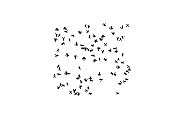
# plot the hexagons with the centers
plot(st_geometry(h3_cells))
plot(h3_centers, pch = 16, add = TRUE, col = "black")
H3Edge vectors representing the boundaries of H3 cells
can be created with h3_edges(),
h3_shared_edge_pairwise(), and
h3_shared_edge_sparse().
cell_edges <- h3_edges(h3s[1:3])
cell_edges
#> [[1]]
#> <H3Edge[6]>
#> [1] 1141f843ffffffff 1241f843ffffffff 1341f843ffffffff 1441f843ffffffff
#> [5] 1541f843ffffffff 1641f843ffffffff
#>
#> [[2]]
#> <H3Edge[6]>
#> [1] 11439723ffffffff 12439723ffffffff 13439723ffffffff 14439723ffffffff
#> [5] 15439723ffffffff 16439723ffffffff
#>
#> [[3]]
#> <H3Edge[6]>
#> [1] 1141843dffffffff 1241843dffffffff 1341843dffffffff 1441843dffffffff
#> [5] 1541843dffffffff 1641843dffffffff
We’ve created a list of each cell’s edges. We can flatten them using
flatten_edges().
cell_edges <- flatten_edges(cell_edges)
cell_edges
#> <H3Edge[18]>
#>  [1] 1141f843ffffffff 1241f843ffffffff 1341f843ffffffff 1441f843ffffffff
#>  [5] 1541f843ffffffff 1641f843ffffffff 11439723ffffffff 12439723ffffffff
#>  [9] 13439723ffffffff 14439723ffffffff 15439723ffffffff 16439723ffffffff
#> [13] 1141843dffffffff 1241843dffffffff 1341843dffffffff 1441843dffffffff
#> [17] 1541843dffffffff 1641843dffffffff
These can be cast to sfc objects using st_as_sfc().
st_as_sfc(cell_edges)
#> Geometry set for 18 features
#> Geometry type: LINESTRING
#> Dimension:     XY
#> Bounding box:  xmin: -4.577141 ymin: 40.10303 xmax: 6.908627 ymax: 48.92561
#> Geodetic CRS:  WGS 84
#> First 5 geometries:
#> LINESTRING (6.828196 48.56718, 6.908627 48.78762)
#> LINESTRING (6.24713 48.62253, 6.49798 48.48486)
#> LINESTRING (6.49798 48.48486, 6.828196 48.56718)
#> LINESTRING (6.656859 48.92561, 6.325574 48.84283)
#> LINESTRING (6.908627 48.78762, 6.656859 48.92561)
Additionally, you can get the vertexes of H3 cell indexes using
h3_to_vertexes() which returns an
sfc_MULTIPOINT.
h3_to_vertexes(h3s)
#> Geometry set for 100 features
#> Geometry type: MULTIPOINT
#> Dimension:     XY
#> Bounding box:  xmin: -5.162291 ymin: 40.02598 xmax: 10.1164 ymax: 50.08041
#> Geodetic CRS:  WGS 84
#> First 5 geometries:
#> MULTIPOINT ((6.325574 48.84283), (6.24713 48.62...
#> MULTIPOINT ((-0.6690999 40.57641), (-0.9475784 ...
#> MULTIPOINT ((-4.227092 46.53696), (-4.535994 46...
#> MULTIPOINT ((1.905903 40.46739), (1.849434 40.2...
#> MULTIPOINT ((8.142693 44.78613), (8.062234 44.5...Since h3o is written in Rust, it is very fast.
h3_strs <- as.character(h3s)
bench::mark(
  h3o = st_as_sfc(h3s),
  h3jsr = h3jsr::cell_to_polygon(h3_strs)
)
#> # A tibble: 2 × 6
#>   expression      min   median `itr/sec` mem_alloc `gc/sec`
#>   <bch:expr> <bch:tm> <bch:tm>     <dbl> <bch:byt>    <dbl>
#> 1 h3o         462.6µs  505.7µs     1863.    9.85KB     14.6
#> 2 h3jsr 8.34ms 9.36ms 106. 2.7MB 90.0nc <- st_read(system.file("gpkg/nc.gpkg", package = "sf"), quiet = TRUE) |>
st_transform(4326) |>
st_geometry()
bench::mark(
h3o = sfc_to_cells(nc, 5, "centroid"),
h3jsr = h3jsr::polygon_to_cells(nc, 5),
check = FALSE
)
#> # A tibble: 2 × 6
#> expression min median `itr/sec` mem_alloc `gc/sec`
#> <bch:expr> <bch:tm> <bch:tm> <dbl> <bch:byt> <dbl>
#> 1 h3o 4.8ms 5.35ms 183. 21.4KB 11.3
#> 2 h3jsr 27.6ms 28.51ms 34.8 748.7KB 4.97bench::mark(
h3o = h3_from_points(pnts$geometry, 3),
h3jsr = h3jsr::point_to_cell(pnts$geometry, 3),
check = FALSE
)
#> # A tibble: 2 × 6
#> expression min median `itr/sec` mem_alloc `gc/sec`
#> <bch:expr> <bch:tm> <bch:tm> <dbl> <bch:byt> <dbl>
#> 1 h3o 103.4µs 123.3µs 7372. 848B 11.4
#> 2 h3jsr 2.63ms 3.04ms 326. 975KB 13.3bench::mark(
h3o = h3_edges(h3s),
h3jsr = h3jsr::get_udedges(h3_strs),
check = FALSE
)
#> # A tibble: 2 × 6
#> expression min median `itr/sec` mem_alloc `gc/sec`
#> <bch:expr> <bch:tm> <bch:tm> <dbl> <bch:byt> <dbl>
#> 1 h3o 403.5µs 530.3µs 1593. 848B 16.9
#> 2 h3jsr 1.64ms 1.76ms 555. 67.9KB 17.3# get edges for a single location
eds <- h3_edges(h3s[1])[[1]]
# strings for h3jsr
eds_str <- as.character(eds)
bench::mark(
h3o = h3_edge_cells(eds),
h3jsr = h3jsr::get_udends(eds_str),
check = FALSE
)
#> # A tibble: 2 × 6
#> expression min median `itr/sec` mem_alloc `gc/sec`
#> <bch:expr> <bch:tm> <bch:tm> <dbl> <bch:byt> <dbl>
#> 1 h3o 12.9µs 18.1µs 49775. 7.86KB 19.9
#> 2 h3jsr 631.3µs 740.1µs 1248. 19.82KB 12.9These binaries (installable software) and packages are in development.
They may not be fully stable and should be used with caution. We make no claims about them.
Health stats visible at Monitor.