

The hardware and bandwidth for this mirror is donated by dogado GmbH, the Webhosting and Full Service-Cloud Provider. Check out our Wordpress Tutorial.
If you wish to report a bug, or if you are interested in having us mirror your free-software or open-source project, please feel free to contact us at mirror[@]dogado.de.
ggtintshade is an extension to the ggplot2
plotting library that allows for the tint/shade of a color to be mapped
to an aesthetic in addition to its hue. This permits visual grouping of
similar points in color space while still allowing a color legend to
disambiguate them overall. It supports both nested and crossed
designs.
You can install the most recent stable version of ggtintshade from CRAN (soon!) as follows:
install.packages("ggtintshade")Alternatively, you can install the development version from GitHub with:
# install.packages("devtools")
devtools::install_github("wkumler/ggtintshade")The original inspiration behind ggtintshade came from
metabolomics experiments where I wanted to be able to discuss both
individual compounds as well as the groups they fell into. A useful
visual guide for this is to have all of one compound type be a single
color, while individual compounds within that group have different
shades.
library(ggtintshade)

metab_data <- data.frame(
  metab = rep(c("Alanine", "Threonine", "Glycine",
                "Glycine betaine", "Proline betaine", "Carnitine",
                "DMSP", "DMS-Ac", "Isethionate"), 3),
  metab_group = rep(rep(c("Amino acid", "Betaine", "Sulfur"), each = 3), 3),
  tripl = rep(c("A", "B", "C"), each = 9),
  area  = runif(27)
)
metab_data$metab <- factor(metab_data$metab, levels = unique(metab_data$metab))

ggplot(metab_data) +
  geom_col_tintshade(aes(x=tripl, y=area, fill=metab_group, tintshade = metab))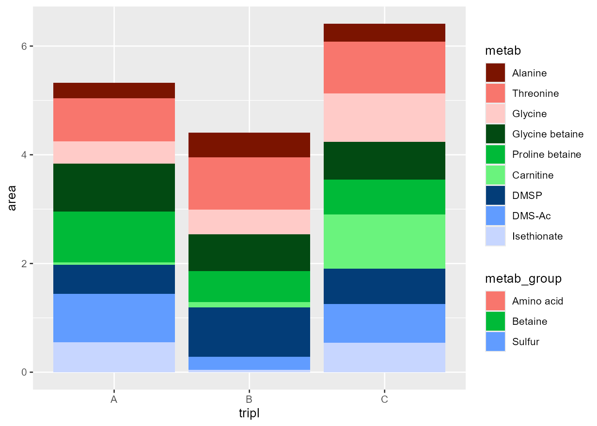
This is a nice example of nested data, where each
individual entry belongs to a single group. ggtintshade
also handles crossed data, where each shade should map
into multiple groups. A good example of this is your D&D-style
“alignment” chart.
align_data <- data.frame(
  alignment=1:9,
  moral=rep(c("good", "neutral", "evil"), each=3),
  meta=rep(c("lawful", "neutral", "chaotic"), length.out=9)
)
align_data$moral <- factor(align_data$moral, levels=rev(unique(align_data$moral)))
align_data$meta <- factor(align_data$meta, levels=unique(align_data$meta))

ggplot(align_data) +
  geom_raster_tintshade(aes(x=meta, y=moral, fill=meta, tintshade=moral)) +
  scale_fill_manual(breaks = c("lawful", "neutral", "chaotic"), values=c("#cca40a", "#b52060", "#7623b2")) +
  coord_equal()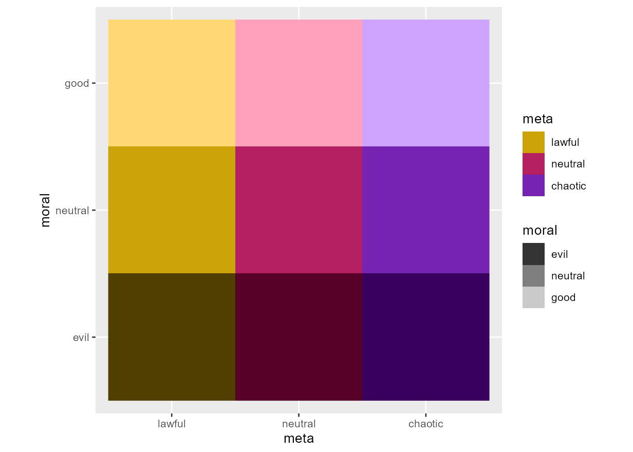
That last plot also demonstrates how well ggtintshade
handles normal ggplot2 behavior. Manually specified colors
are handled naturally and the interaction is seamless, but you can also
control the degree of lightening/darkening using the expected
ggplot2 syntax for the new aesthetic with the associated
scale. For example, using the diamonds dataset:
grp <- c(I1 = "I", SI2 = "SI", SI1 = "SI", VS2 = "VS", VS1 = "VS", VVS2 = "VVS", VVS1 = "VVS", IF = "IF")
diamonds$clarity_group <- factor(grp[as.character(diamonds$clarity)], levels = c("I", "SI", "VS", "VVS", "IF"))
mp <- aggregate(price ~ clarity + clarity_group, diamonds, mean)

crossed_gp <- ggplot(mp) +
  geom_col_tintshade(aes(clarity, price, fill = clarity_group, tintshade = clarity)) +
  scale_tintshade_discrete(range = c(0.4, 0.6)) +
  ggtitle("Nested diamonds") +
  theme(axis.text.x = element_text(angle=90, hjust=1, vjust=0.5))
nested_gp <- ggplot(diamonds) +
  geom_bar_tintshade(aes(x=cut, fill = cut, tintshade = clarity), color="black") +
  ggtitle("Crossed diamonds") +
  scale_tintshade_discrete(range = c(0.1, 0.9)) +
  theme(axis.text.x = element_text(angle=90, hjust=1, vjust=0.5))
crossed_gp + nested_gp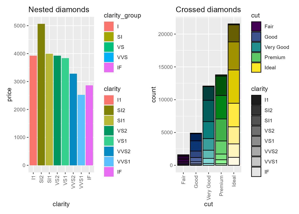
This package is a much better way to map a lightness aesthetic than
the advice commonly offered online to use alpha instead.
(e.g here, here, here and here)
For one, alpha only lightens, not darkens, and creates an unhelpful
transparency that must be handled. It also avoids having to calculate an
interaction and then set a manual scale for two aesthetics pasted
together. Additionally, using an overlapping alpha trace is inefficient
and can cause issues if exported to a vectorized format because each
point has multiple values.
For example, solving the question raised in Different color shades for faceted grouped bar plots in ggplot2:
temp.data = data.frame (
  Species  = rep(c("A","B"),each=2, times=2),
  Status = rep(c("An","Bac"), times=4),
  Sex = rep(c("Male","Female"), each=4, times=1),
  Proportion = c(6.86, 7.65, 30.13, 35.71, 7.13, 10.33, 29.24, 31.09)
)
init_alpha <- ggplot(temp.data, aes(x = Species, y = Proportion, fill = Status, alpha = Species)) +
  geom_bar(stat='identity', position = position_dodge(width = 0.73), width=.67) +
  facet_grid(Sex ~ .) +
  scale_fill_manual(name = "Status", labels = c("An","Bac"), values = c("#86a681","#0a3e03")) +
  ggtitle("Without ggtintshade")
new_tinted <- ggplot(temp.data, aes(x = Species, y = Proportion, fill = Species, tintshade = Status)) +
  geom_bar_tintshade(stat='identity', position = position_dodge(width = 0.73), width=.67) +
  facet_grid(Sex ~ .) +
  scale_fill_manual(name = "Status", labels = c("An","Bac"), values = c("#cf944c","#0a3e03")) +
  scale_tintshade_discrete(range = c(0.3, 0.7)) +
  ggtitle("With ggtintshade")
init_alpha + new_tinted
#> Warning: Using alpha for a discrete variable is not advised.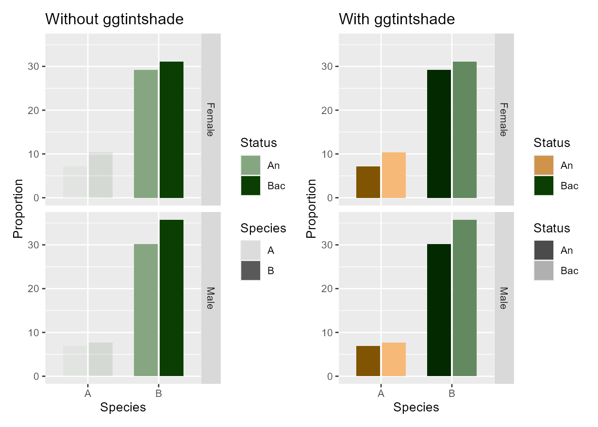
Or the question here (grouping multiple gradients using ggplot2) which also demonstrates a continuous tint gradient (and why alpha is a bad idea when points overlap!):
d <- data.frame(
  x=rep(1:20, 5), y=rnorm(100, 5, .2) + rep(1:5, each=20),
  z=rep(1:20, 5), grp=factor(rep(1:5, each=20))
)

init_alpha <- ggplot(d) +
  geom_path(aes(x, y, color=grp), linewidth=2, lineend=0) +
  geom_path(aes(x, y, group=grp, alpha=z), linewidth=2, lineend=0) +
  ggtitle("Without ggtintshade")
new_tinted <- ggplot(d) +
  geom_path_tintshade(aes(x, y, color=grp, tintshade=z), linewidth=2, lineend=0) +
  scale_tintshade_continuous(range = c(0.5, 0)) +
  ggtitle("With ggtintshade")
init_alpha + new_tinted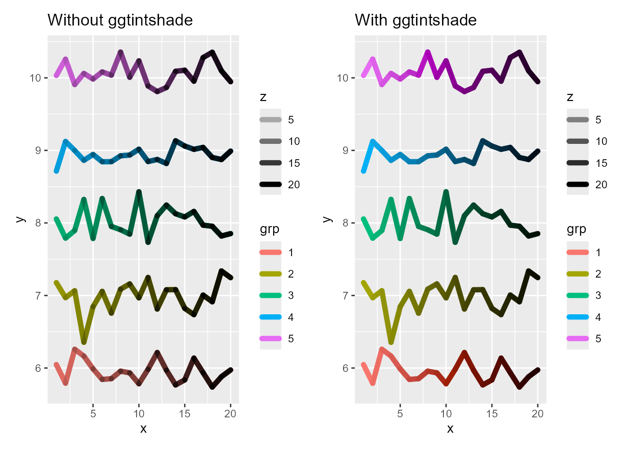
mpgsub <- head(mpg, 60)
mpgsub$model <- factor(mpgsub$model, levels=unique(mpgsub$model))
ggplot(mpgsub, aes(displ, hwy, colour = manufacturer, tintshade = model)) +
  geom_point_tintshade(size = 3)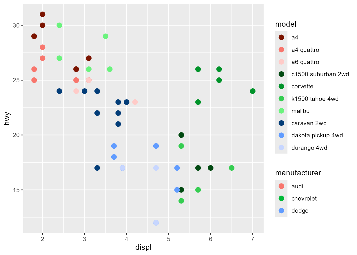
ggplot(penguins) +
  geom_point_tintshade(aes(x=bill_len, y=bill_dep, fill=species, tintshade=sex),
                       pch=21, color="black", size=3)
#> Warning: Removed 2 rows containing missing values or values outside the scale range
#> (`geom_point_tintshade()`).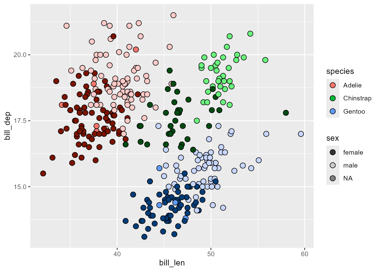
This last example also shows how NA tintshade values are mapped to the untinted shade, which could cause some confusion. The recommended approach in this case is to ensure that the NA values are also mapped to an additional aesthetic, e.g. shape.
Internally, this is a bit of a hack. Base ggplot2 treats
each aesthetic separately and does not like allowing them to interact in
this way. We get around this issue first by creating a cache that’s
passed around in the ggproto object and then we (ab)use the
use_defaults step where all the necessary information is
available. For more details about this, see the [internals
vignette].
ggtintshade uses colorspace::lighten to
actually modify the colors, so review the documentation there for more
information about how the color values are remapped.
The individual geoms are generated via a factory [R/geoms.R] instead
of copy-pasting code, so adding new geoms isn’t difficult as long as
they inherit naturally from an existing ggplot2
function.
Issues: https://github.com/wkumler/ggtintshade/issues
README last built on 2026-07-15
These binaries (installable software) and packages are in development.
They may not be fully stable and should be used with caution. We make no claims about them.
Health stats visible at Monitor.