README

The hardware and bandwidth for this mirror is donated by dogado GmbH, the Webhosting and Full Service-Cloud Provider. Check out our Wordpress Tutorial.
If you wish to report a bug, or if you are interested in having us mirror your free-software or open-source project, please feel free to contact us at mirror[@]dogado.de.

ggstats: extension to ggplot2 for plotting stats

The ggstats package provides new statistics, new geometries and new positions for ggplot2 and a suite of functions to facilitate the creation of statistical plots.

Installation & Documentation

install.packages("ggstats")

remotes::install_github("larmarange/ggstats")

Plot model coefficients

library(ggstats)

mod1 <- lm(Fertility ~ ., data = swiss)
ggcoef_model(mod1)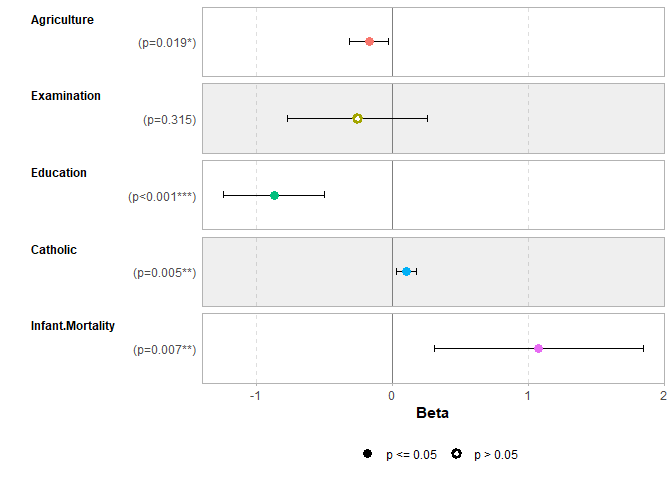

ggcoef_table(mod1)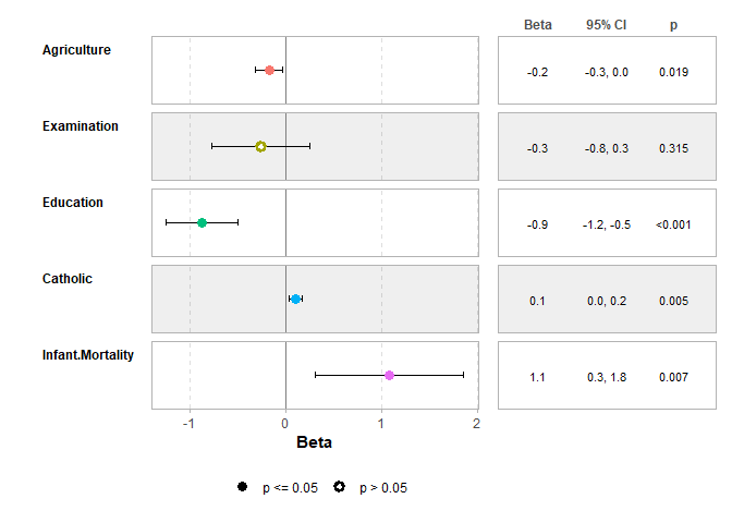

Comparing several models

mod2 <- step(mod1, trace = 0)
mod3 <- lm(Fertility ~ Agriculture + Education * Catholic, data = swiss)
models <- list(
  "Full model" = mod1,
  "Simplified model" = mod2,
  "With interaction" = mod3
)

ggcoef_compare(models, type = "faceted")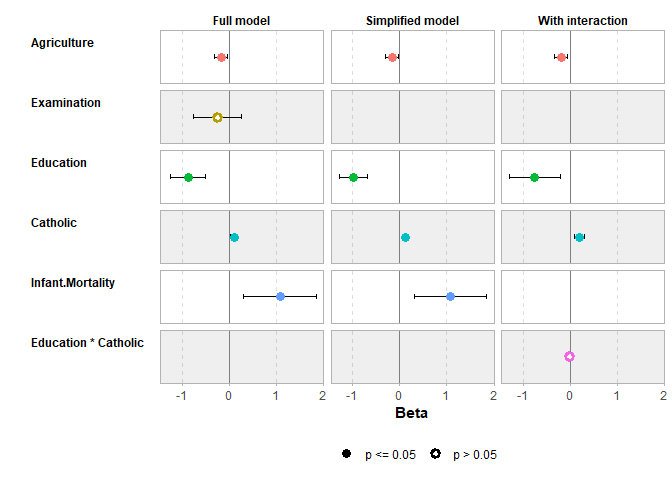

Compute custom proportions

library(ggplot2)
ggplot(as.data.frame(Titanic)) +
  aes(x = Class, fill = Survived, weight = Freq, by = Class) +
  geom_bar(position = "fill") +
  geom_text(stat = "prop", position = position_fill(.5)) +
  facet_grid(~Sex)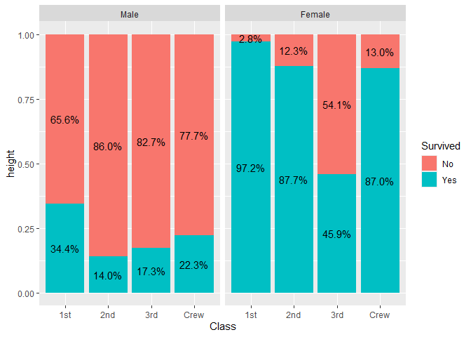

Compute weighted mean

data(tips, package = "reshape")
ggplot(tips) +
  aes(x = day, y = total_bill, fill = sex) +
  stat_weighted_mean(geom = "bar", position = "dodge") +
  ylab("Mean total bill per day and sex")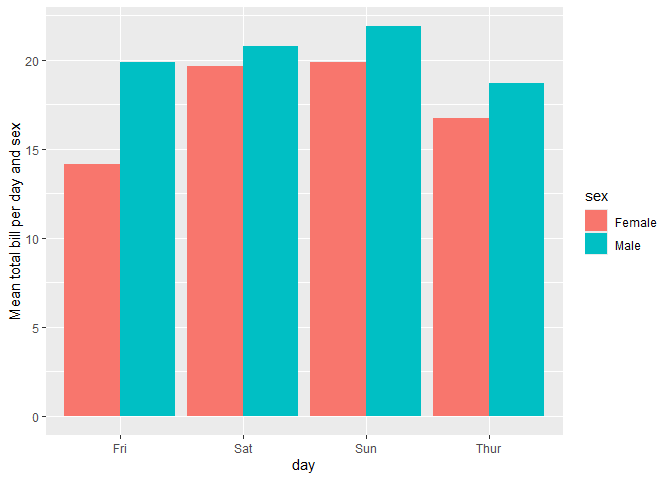

Compute cross-tabulation statistics

ggplot(as.data.frame(Titanic)) +
  aes(
    x = Class, y = Survived, weight = Freq,
    size = after_stat(observed), fill = after_stat(std.resid)
  ) +
  stat_cross(shape = 22) +
  scale_fill_steps2(breaks = c(-3, -2, 2, 3), show.limits = TRUE) +
  scale_size_area(max_size = 20)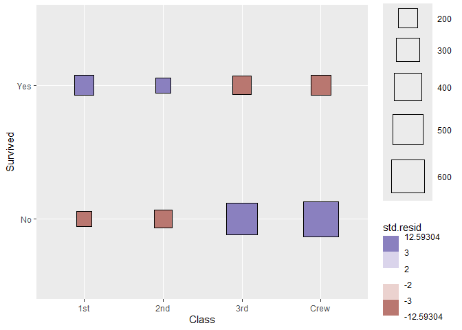

Plot survey objects taking into account weights

library(survey, quietly = TRUE)
#> 
#> Attachement du package : 'survey'
#> L'objet suivant est masqué depuis 'package:graphics':
#> 
#>     dotchart
dw <- svydesign(
  ids = ~1,
  weights = ~Freq,
  data = as.data.frame(Titanic)
)
ggsurvey(dw) +
  aes(x = Class, fill = Survived) +
  geom_bar(position = "fill") +
  ylab("Weighted proportion of survivors")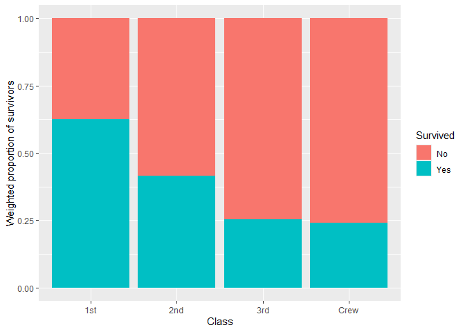

Plot Likert-type items

library(dplyr)
#> 
#> Attachement du package : 'dplyr'
#> Les objets suivants sont masqués depuis 'package:stats':
#> 
#>     filter, lag
#> Les objets suivants sont masqués depuis 'package:base':
#> 
#>     intersect, setdiff, setequal, union
likert_levels <- c(
  "Strongly disagree",
  "Disagree",
  "Neither agree nor disagree",
  "Agree",
  "Strongly agree"
)
set.seed(42)
df <-
  tibble(
    q1 = sample(likert_levels, 150, replace = TRUE),
    q2 = sample(likert_levels, 150, replace = TRUE, prob = 5:1),
    q3 = sample(likert_levels, 150, replace = TRUE, prob = 1:5),
    q4 = sample(likert_levels, 150, replace = TRUE, prob = 1:5),
    q5 = sample(c(likert_levels, NA), 150, replace = TRUE),
    q6 = sample(likert_levels, 150, replace = TRUE, prob = c(1, 0, 1, 1, 0))
  ) |>
  mutate(across(everything(), ~ factor(.x, levels = likert_levels)))

gglikert(df)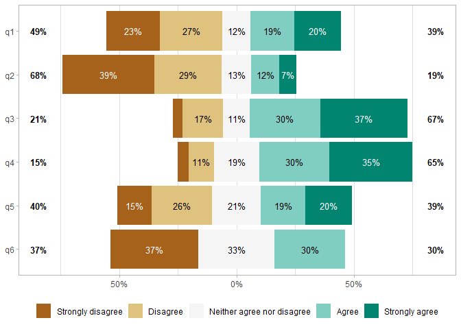

Connect bars

ggplot(diamonds) +
  aes(x = clarity, fill = cut) +
  geom_bar(width = .5) +
  geom_bar_connector(width = .5, linewidth = .25) +
  theme_minimal() +
  theme(legend.position = "bottom")

Generate a cascade plot

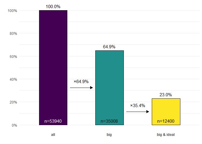
diamonds |>
  ggcascade(
    all = TRUE,
    big = carat > .5,
    "big & ideal" = carat > .5 & cut == "Ideal"
  )

These binaries (installable software) and packages are in development.
They may not be fully stable and should be used with caution. We make no claims about them.
Health stats visible at Monitor.

ggstats: extension to ggplot2 for plotting stats