The hardware and bandwidth for this mirror is donated by dogado GmbH, the Webhosting and Full Service-Cloud Provider. Check out our Wordpress Tutorial.
If you wish to report a bug, or if you are interested in having us mirror your free-software or open-source project, please feel free to contact us at mirror[@]dogado.de.

![]()
![]()

![]()
![]()
Neuroimaging analyses produce region-level results – cortical thickness, p-values, network assignments – that need to end up on a brain figure. ggseg stores brain atlas geometries as simple features and plots them as ggplot2 layers, so you get publication-ready brain figures with the same code you’d use for any other ggplot.
Mowinckel & Vidal-Piñeiro (2020). Visualization of Brain Statistics With R Packages ggseg and ggseg3d. Advances in Methods and Practices in Psychological Science.
Install from CRAN:
install.packages("ggseg")Or get the development version from the ggsegverse r-universe:
options(repos = c(
  ggsegverse = "https://ggsegverse.r-universe.dev",
  CRAN = "https://cloud.r-project.org"
))
install.packages("ggseg")library(ggseg)
library(ggplot2)ggseg ships with three atlases: dk (Desikan-Killiany
cortical parcellation), aseg (automatic subcortical
segmentation), and tracula (white matter tracts).
plot() gives you a quick overview:
plot(dk())
plot(aseg())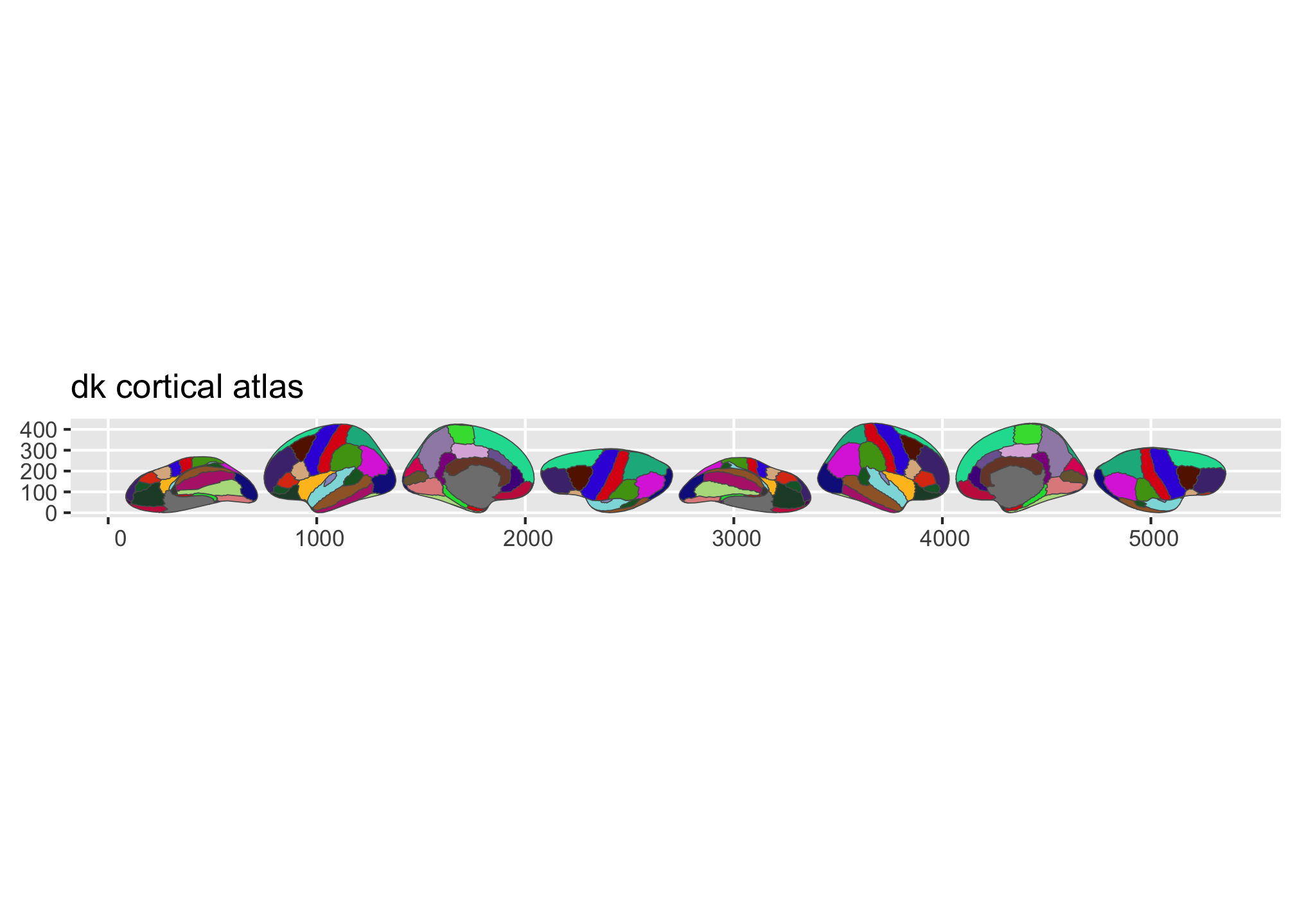
Figure 1: Overview of the dk and aseg built-in brain atlases.
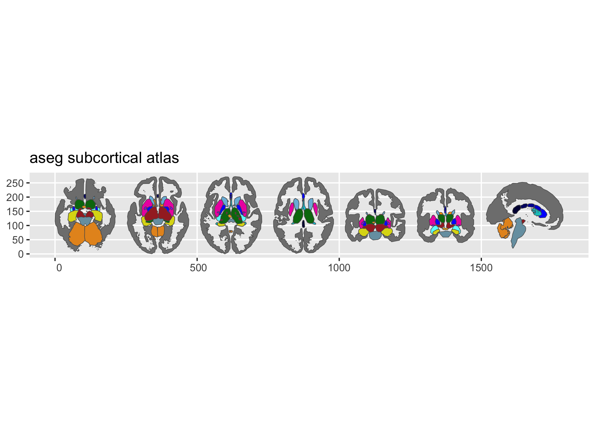
Figure 2: Overview of the dk and aseg built-in brain atlases.
Pass a data frame to ggplot() with a column that matches
the atlas (typically region or label).
geom_brain() handles the join:
library(dplyr)

some_data <- tibble(
  region = rep(
    c(
      "transverse temporal",
      "insula",
      "precentral",
      "superior parietal"
    ),
    2
  ),
  p = sample(seq(0, .5, .001), 8),
  groups = c(rep("g1", 4), rep("g2", 4))
)

ggplot(some_data) +
  geom_brain(
    atlas = dk(),
    position = position_brain(hemi ~ view),
    aes(fill = p)
  ) +
  facet_wrap(~groups) +
  scale_fill_viridis_c(option = "cividis", direction = -1) +
  theme_void()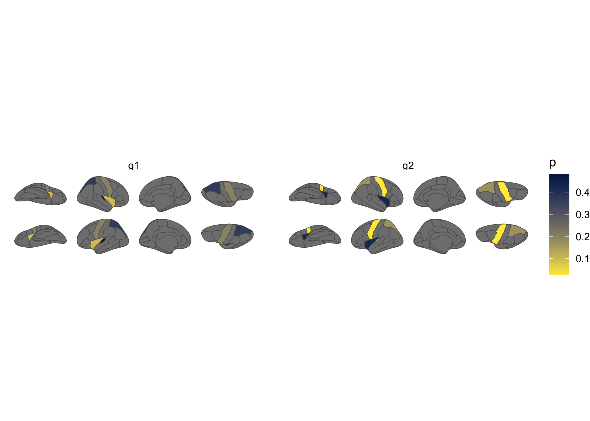
Figure 3: Brain plot coloured by external data, faceted by group.
Many additional atlases are available through the ggsegverse r-universe:
install.packages("ggsegYeo2011", repos = "https://ggsegverse.r-universe.dev")The package website
has vignettes covering external data, view positioning, the
geom_sf() workflow, and reading FreeSurfer stats files.
This tool is partly funded by:
EU Horizon 2020 Grant: Healthy minds 0-100 years: Optimising the use of European brain imaging cohorts (Lifebrain). Grant agreement number: 732592.
These binaries (installable software) and packages are in development.
They may not be fully stable and should be used with caution. We make no claims about them.
Health stats visible at Monitor.