The hardware and bandwidth for this mirror is donated by dogado GmbH, the Webhosting and Full Service-Cloud Provider. Check out our Wordpress Tutorial.
If you wish to report a bug, or if you are interested in having us mirror your free-software or open-source project, please feel free to contact us at mirror[@]dogado.de.

ggmeta

ggmeta builds publication-quality forest and funnel plots with ggplot2. Give it a meta object (from the meta package) or a plain tidy data frame — the result is an ordinary ggplot you can theme, compose, and save.

Installation

# install.packages("remotes")
remotes::install_github("drhrf/ggmeta")

Quick start

No meta package required — a tidy data frame of effect sizes and standard errors is enough. Set add_summary = TRUE to pool the studies on the fly (inverse-variance common effect and DerSimonian–Laird random effects):

library(ggmeta)

studies <- data.frame(
  studlab  = c("Trial 1", "Trial 2", "Trial 3", "Trial 4", "Trial 5"),
  estimate = c(0.10, 0.35, 0.22, 0.48, 0.05),
  se       = c(0.12, 0.10, 0.14, 0.16, 0.11)
)
studies$ci_lower <- studies$estimate - 1.96 * studies$se
studies$ci_upper <- studies$estimate + 1.96 * studies$se

ggforest(studies, add_summary = TRUE)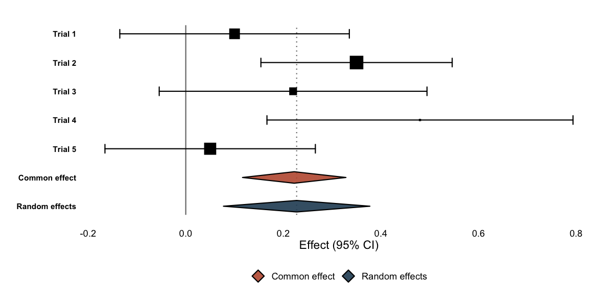

Estimates, CIs, weights, and heterogeneity

Pass a meta object and add columns = TRUE to reproduce the familiar meta::forest() table: an effect estimate, 95% CI, and weight column for every study and summary, headers, and a heterogeneity line (I², the between-study variance, Q, and p) — all as a plain ggplot.

library(meta)
#> Loading required package: metabook
#> Loading 'meta' package (version 8.5-0).
#> Type 'help(meta)' for a brief overview.

dat <- data.frame(
  study   = c("Adams 2019", "Baker 2020", "Chen 2020",
              "Diaz 2021", "Evans 2022", "Foster 2023"),
  event.e = c(12,  8, 25, 18, 30, 15), n.e = c(120,  90, 200, 150, 250, 130),
  event.c = c(20, 14, 30, 28, 35, 25), n.c = c(118,  92, 205, 148, 245, 128)
)

m <- metabin(event.e, n.e, event.c, n.c,
             data = dat, studlab = study, sm = "RR")

ggforest(m, columns = TRUE)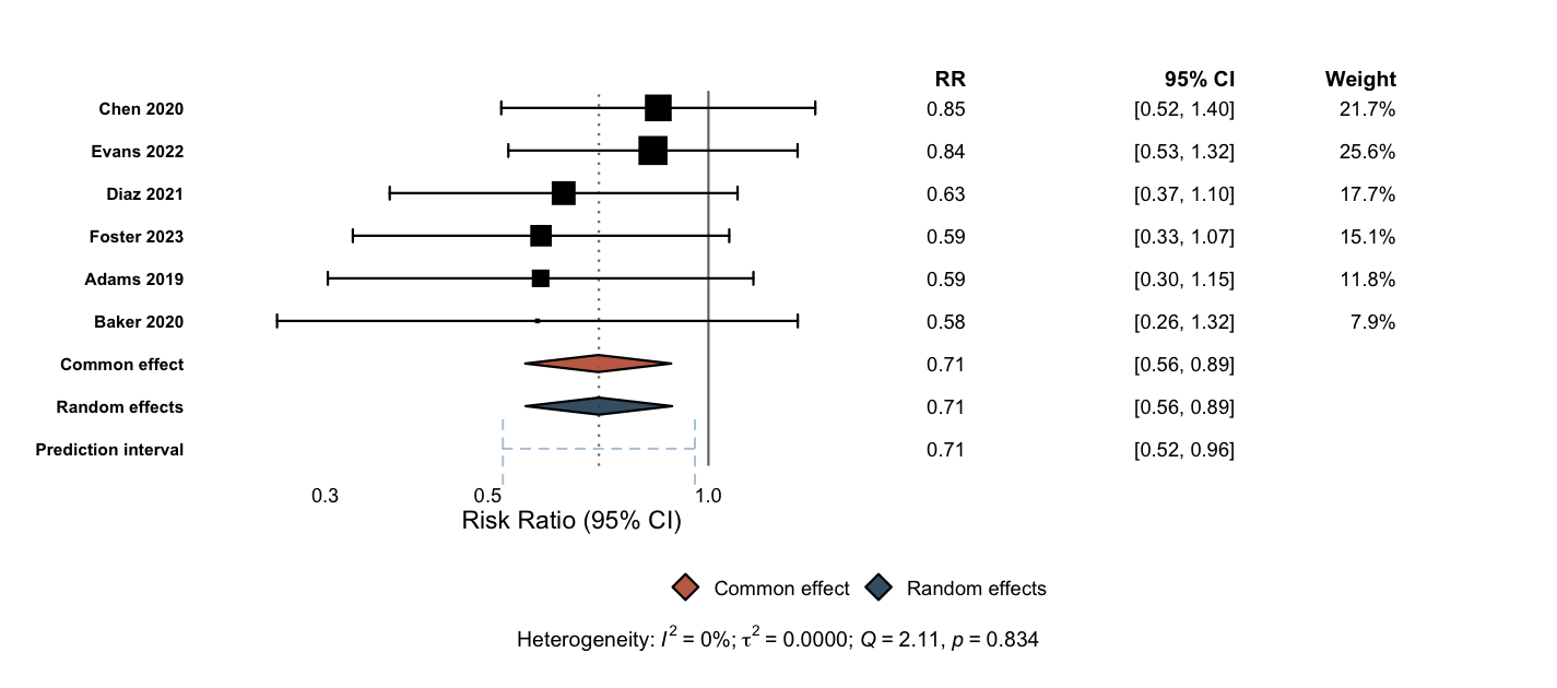

Everything is optional. Choose which columns to show, and toggle the other elements on or off:

ggforest(m, columns = c("estimate", "ci")) # only some columns
ggforest(m, effect_header = "Risk ratio")  # rename the estimate column
ggforest(m, show_hetstats = FALSE)          # hide the heterogeneity line
ggforest(m, show_predict  = FALSE)          # hide the prediction interval
ggforest(m, sort_studies  = FALSE)          # keep the input order

Forest and funnel plots on one canvas

ggmeta also draws funnel plots with ggfunnel() (study effect vs. standard error, with pseudo confidence-interval contours). And because every plot is an ordinary ggplot, a forest and a funnel compose on a single figure with patchwork — something that is awkward with the base-graphics output of meta:

library(patchwork)

(ggforest(m) | ggfunnel(m)) +
  plot_layout(widths = c(2, 1)) +
  plot_annotation(tag_levels = "A")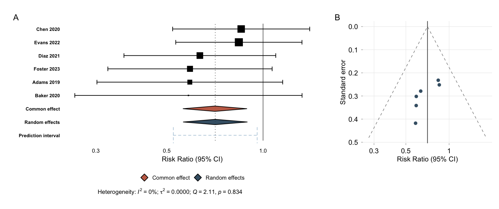

Journal styles

Layout presets restyle a plot for common journals. They are ordinary ggplot2 components, so you add them with +:

layout_jama(ggforest(m, columns = TRUE))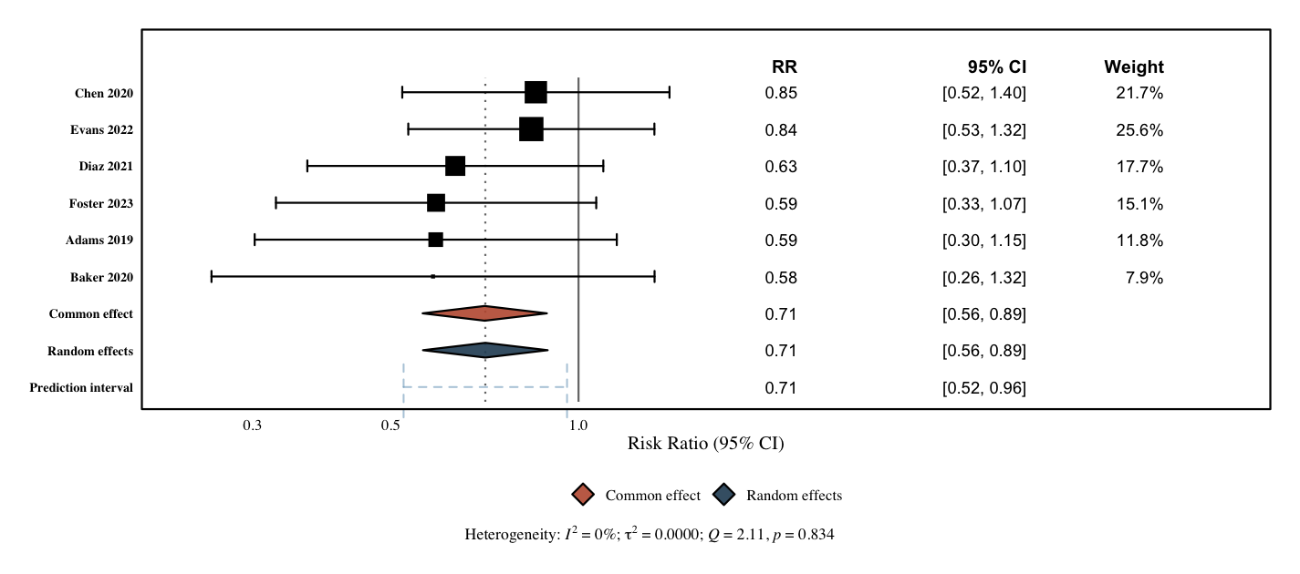

layout_bmj() and layout_revman5() are also available.

Custom columns

For a column of your own — sample sizes, events, anything — use geom_forest_text(), aligned to the study rows through the shared y. tidy_meta() exposes the same tidy data frame ggforest() builds internally, and format_effect() builds "estimate (low to high)" labels:

td      <- tidy_meta(m)
studies <- td[!td$is_summary, ]

ggforest(m) +
  geom_forest_text(aes(y = studlab, label = n.e), data = studies,
                   x = 4, hjust = 0) +
  expand_limits(x = 6)

Why ggmeta?

• ggplot2 native — add themes, layers, annotations, and facets; save with ggsave().
• Forest and funnel plots — ggforest() and ggfunnel(), both ordinary ggplots, so you can arrange them together with patchwork.
• meta::forest()-style tables — estimate / CI / weight columns and a heterogeneity caption, via columns = TRUE.
• Standalone or meta — works on a tidy data frame or a meta object, and can pool studies itself (add_summary = TRUE).
• Correct by construction — every summary measure is back-transformed with its right inverse (ratios, logit proportions, Fisher-z correlations, rates).
• Custom geometries — proper ggproto geoms for CIs, summary diamonds, prediction intervals, reference lines, and text columns.
• Journal styles — layout_jama(), layout_bmj(), layout_revman5().

Learn more

• vignette("getting-started") — a tour of the package.
• vignette("customising") — restyle every element of a forest or funnel plot.
• vignette("from-meta-forest") — coming from meta::forest().

These binaries (installable software) and packages are in development.
They may not be fully stable and should be used with caution. We make no claims about them.
Health stats visible at Monitor.