
The hardware and bandwidth for this mirror is donated by dogado GmbH, the Webhosting and Full Service-Cloud Provider. Check out our Wordpress Tutorial.
If you wish to report a bug, or if you are interested in having us mirror your free-software or open-source project, please feel free to contact us at mirror[@]dogado.de.
You can install ggdark from GitHub with:
# install.packages("devtools")
devtools::install_github("nsgrantham/ggdark")library(ggplot2)
p <- ggplot(diamonds) +
geom_point(aes(carat, price, color = cut)) +
scale_y_continuous(label = scales::dollar) +
guides(color = guide_legend(reverse = TRUE)) +
labs(title = "Prices of 50,000 round cut diamonds by carat and cut",
x = "Weight (carats)",
y = "Price in US dollars",
color = "Quality of the cut")
p + theme_gray() # ggplot default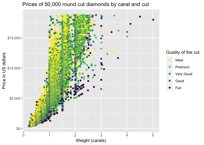
library(ggdark)

p + dark_theme_gray()  # the dark version
#> Inverted geom defaults of fill and color/colour.
#> To change them back, use invert_geom_defaults().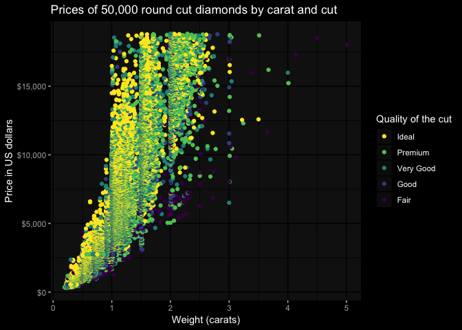
# modify the theme to your liking, as you would in ggplot2
p + dark_theme_gray(base_family = "Fira Sans Condensed Light", base_size = 14) +
  theme(plot.title = element_text(family = "Fira Sans Condensed"),
        plot.background = element_rect(fill = "grey10"),
        panel.background = element_blank(),
        panel.grid.major = element_line(color = "grey30", size = 0.2),
        panel.grid.minor = element_line(color = "grey30", size = 0.2),
        legend.background = element_blank(),
        axis.ticks = element_blank(),
        legend.key = element_blank(),
        legend.position = c(0.815, 0.27))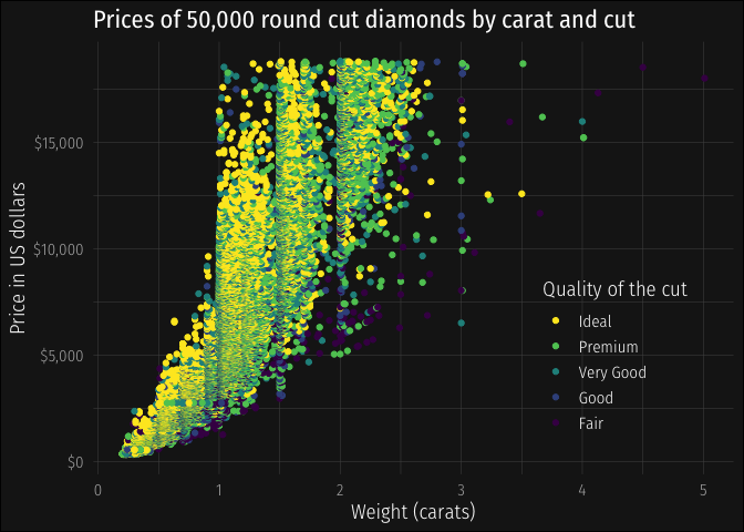
ggdark provides dark versions of all themes available in ggplot2:
mtcars2 <- within(mtcars, {
  vs <- factor(vs, labels = c("V-shaped", "Straight"))
  am <- factor(am, labels = c("Automatic", "Manual"))
  cyl  <- factor(cyl)
  gear <- factor(gear)
})

p <- ggplot(mtcars2) +
  geom_point(aes(wt, mpg, color = gear)) +
  facet_grid(vs ~ am) +
  labs(title = "Fuel economy declines as weight increases",
       subtitle = "(1973-74)",
       caption = "Data from the 1974 Motor Trend US magazine.",
       x = "Weight (1000 lbs)",
       y = "Fuel economy (mpg)",
       color = "Gears")
p + dark_theme_gray()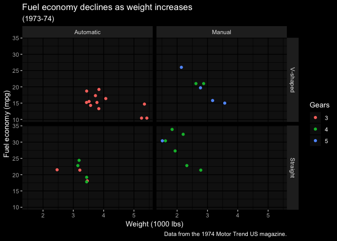
p + dark_theme_bw()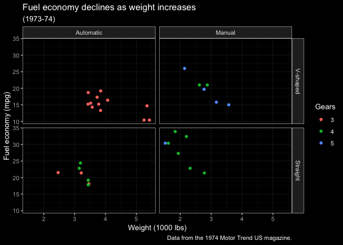
p + dark_theme_linedraw()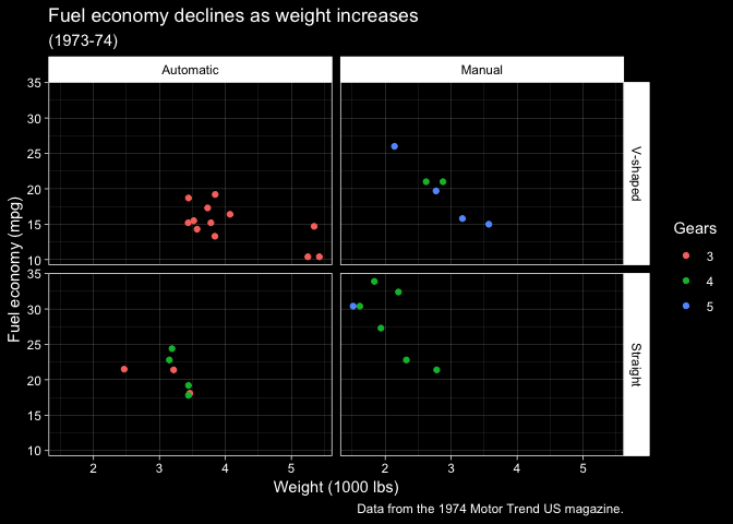
p + dark_theme_light() # quite dark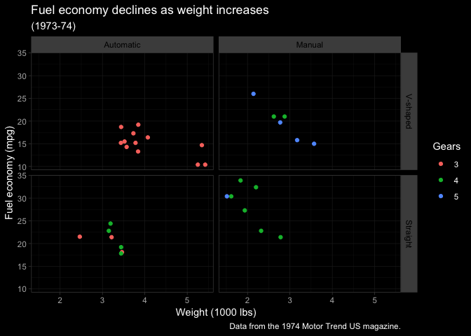
p + dark_theme_dark() # quite light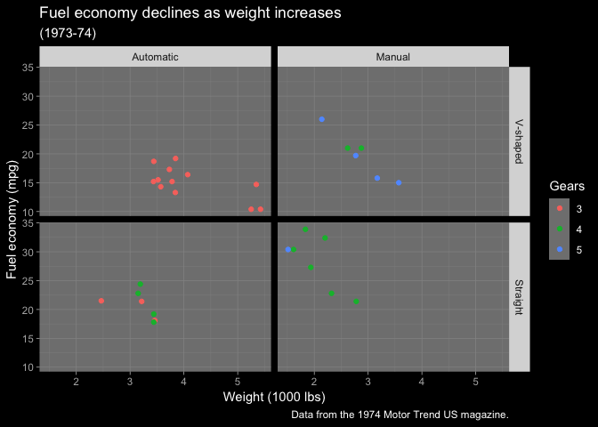
p + dark_theme_minimal()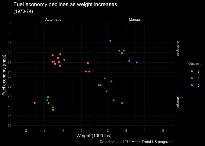
p + dark_theme_classic()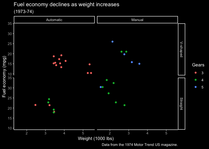
p + dark_theme_void()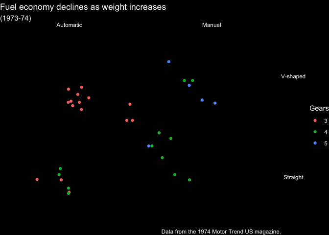
Usedark_mode on any theme to create its dark
version.
invert_geom_defaults()  # change geom defaults back to black

library(gapminder)

p <- ggplot(subset(gapminder, continent != "Oceania")) +
  geom_line(aes(year, lifeExp, group = country, color = country), lwd = 1, show.legend = FALSE) +
  facet_wrap(~ continent) +
  scale_color_manual(values = country_colors) +
  labs(title = "Life expectancy has increased across the globe")
# install.packages("ggthemes")
library(ggthemes)
p + theme_fivethirtyeight()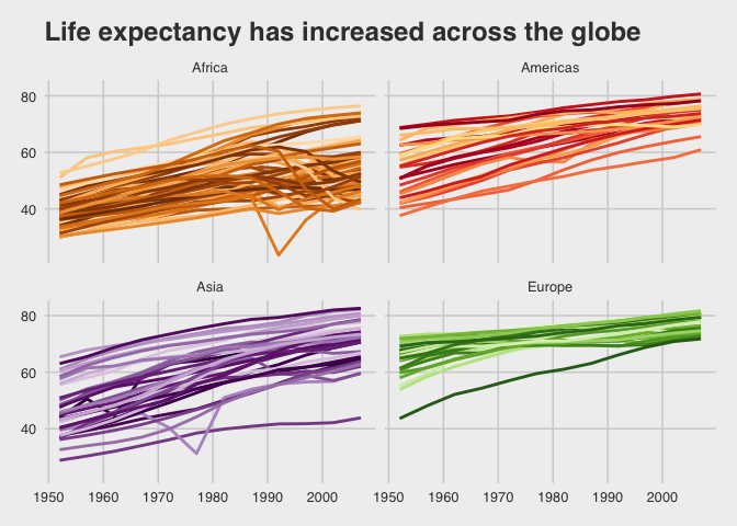
p + dark_mode(theme_fivethirtyeight())
#> Inverted geom defaults of fill and color/colour.
#> To change them back, use invert_geom_defaults().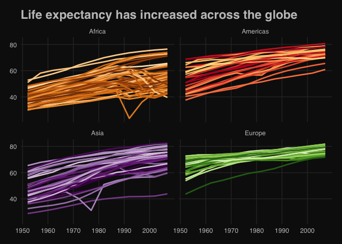
invert_geom_defaults() # leave the geom defaults how you found them!Happy plotting! 🖤
These binaries (installable software) and packages are in development.
They may not be fully stable and should be used with caution. We make no claims about them.
Health stats visible at Monitor.