The hardware and bandwidth for this mirror is donated by dogado GmbH, the Webhosting and Full Service-Cloud Provider. Check out our Wordpress Tutorial.
If you wish to report a bug, or if you are interested in having us mirror your free-software or open-source project, please feel free to contact us at mirror[@]dogado.de.
![]()
![]()
ggcorrheatmap is a convenient package for generating correlation heatmaps made with ggplot2, with support for triangular layouts, clustering and annotation. As the output is a ggplot2 object you can further customise the appearance using familiar ggplot2 functions. Besides correlation heatmaps, there is also support for making general heatmaps.
You can install ggcorrheatmap from CRAN using:
install.packages("ggcorrheatmap")Or you can install the development version from GitHub with:
# install.packages("devtools")
devtools::install_github("leod123/ggcorrheatmap")Below is an example of how to generate a correlation heatmap with clustered rows and columns and row annotation, using a triangular layout that excludes redundant cells.
library(ggcorrheatmap)

set.seed(123)
# Make a correlation heatmap with a triangular layout, annotations and clustering
row_annot <- data.frame(.names = colnames(mtcars),
                        annot1 = sample(letters[1:3], ncol(mtcars), TRUE),
                        annot2 = rnorm(ncol(mtcars)))
ggcorrhm(mtcars, layout = "bottomright",
         cluster_rows = TRUE, cluster_cols = TRUE,
         show_dend_rows = FALSE, annot_rows_df = row_annot)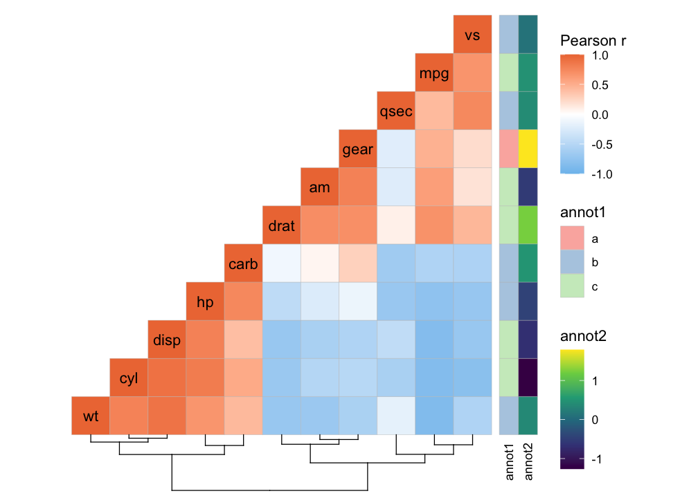
Or a mixed layout that displays different things in the different triangles.
# With correlation values and p-values
ggcorrhm(mtcars, layout = c("topright", "bottomleft"),
         cell_labels = c(FALSE, TRUE), p_values = c(FALSE, TRUE))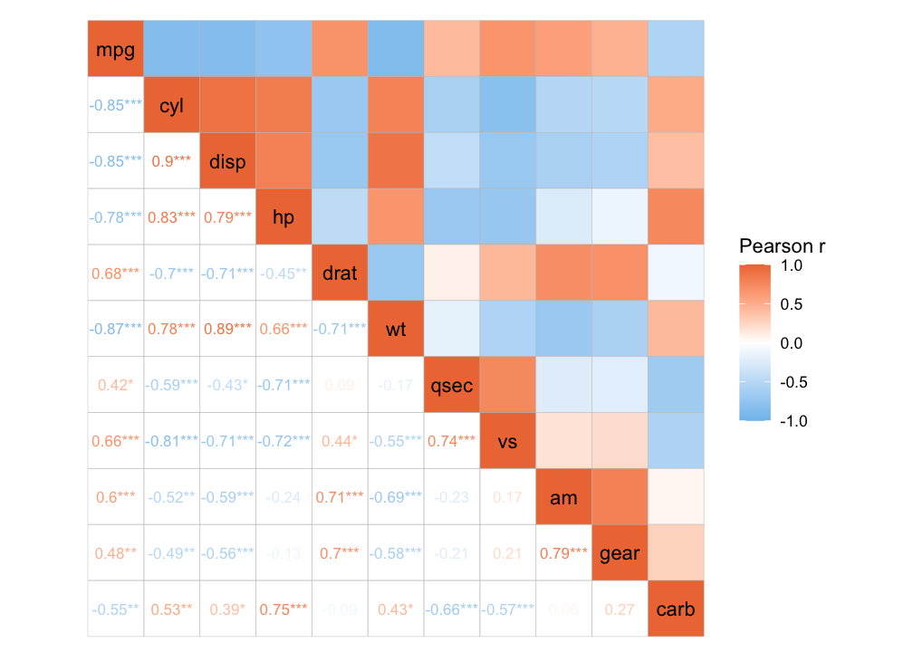
It is also possible to make a normal heatmap, for a more flexible output.
gghm(mtcars, scale_data = "col", cluster_rows = TRUE, cluster_cols = TRUE)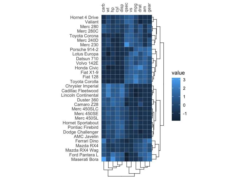
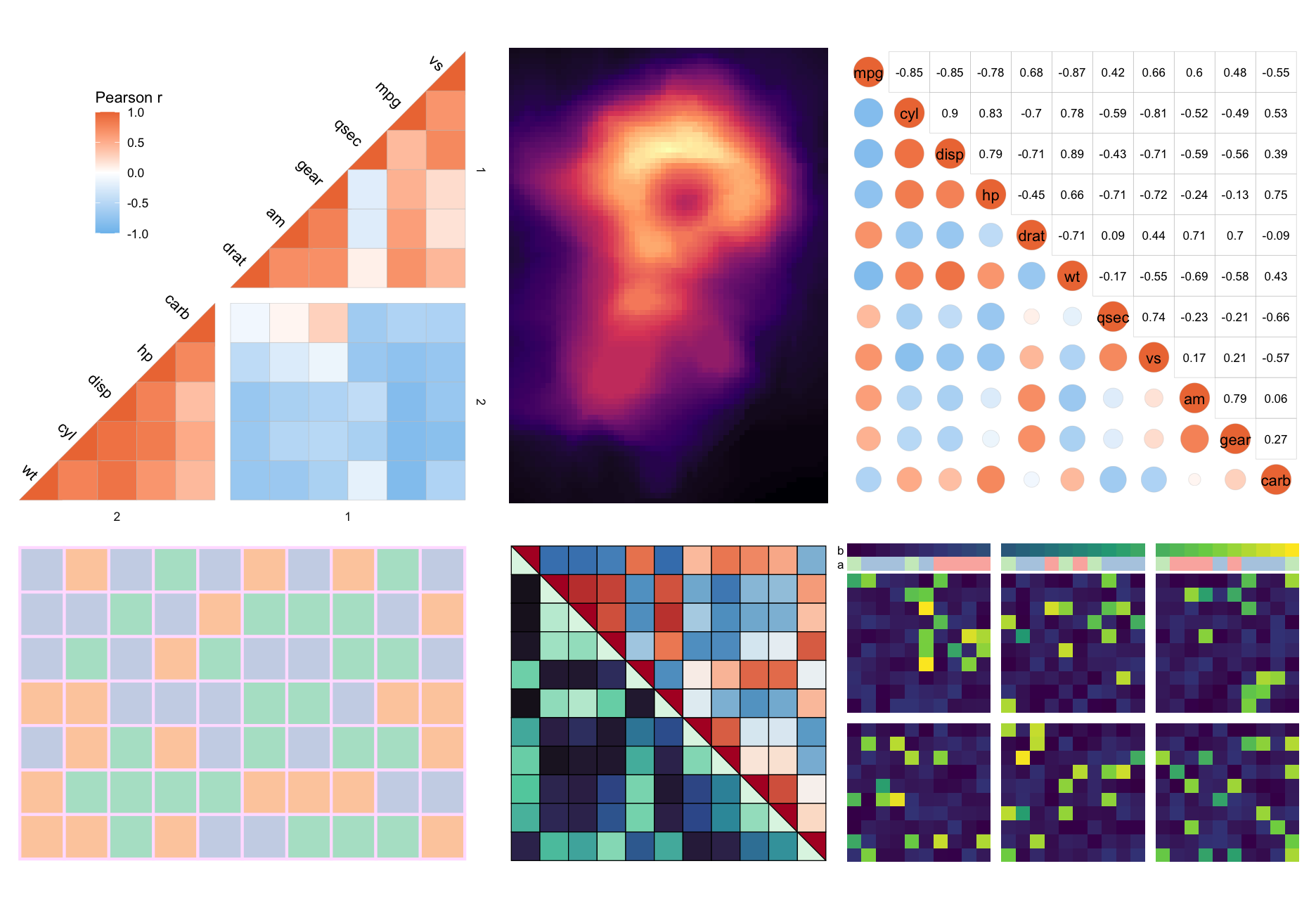
Below is a showcase more things you could do with the package (the code can be found at the bottom).
More examples can be found in the articles of the package:
library(ggplot2)   # moving legend for plot 1
library(patchwork) # for combining into one big figure

# Clustered triangular heatmap with gaps
plt1 <- ggcorrhm(mtcars, layout = "bottomright",
                 split_diag = TRUE,
                 cluster_rows = TRUE, cluster_cols = TRUE,
                 split_rows = 2, split_cols = 2,
                 names_diag_params = list(angle = -45, hjust = 1.3)) +
  theme(legend.position = "inside", legend.position.inside = c(0.25, 0.75))

# Heatmap with other colour scale
plt2 <- gghm(volcano, col_scale = "A", border_col = NA, legend_order = NA,
             show_names_rows = FALSE, show_names_cols = FALSE)

# Mixed correlation heatmap with circles and correlation values
plt3 <- ggcorrhm(mtcars, layout = c("bl", "tr"), mode = c("21", "none"),
                 legend_order = NA, cell_labels = c(FALSE, TRUE))

# Heatmap with categorical values
set.seed(123)
plt4 <- gghm(matrix(letters[sample(1:3, 70, TRUE)], nrow = 7),
             col_scale = "Pastel2", border_col = "#FFE1FF", legend_order = NA,
             border_lwd = 1, show_names_rows = FALSE, show_names_cols = FALSE)

# Split square heatmap with two colour scales
plt5 <- ggcorrhm(mtcars, layout = c("tr", "bl"), mode = c("hm", "hm"),
                 col_scale = c("RdBu_rev", "G"), split_diag = TRUE,
                 border_lwd = 0.3, border_col = 1,
                 legend_order = NA, show_names_diag = FALSE)

# Annotations and gaps
set.seed(123)
dat6 <- sapply(sample(1:5, 30, TRUE), \(x) {
    c(runif(x, runif(1, 0.5, 0.8), runif(1, 0.81, 1)), runif(20 - x, 0, 0.2))[sample(1:20, 20, FALSE)]
})
plt6 <- gghm(dat6, border_col = 0, col_scale = "D",
             show_names_rows = FALSE, show_names_cols = FALSE,
             legend_order = NA, split_rows = 10, split_cols = c(10, 20),
             annot_cols_df = data.frame(a = sample(letters[1:3], 30, TRUE), b = 1:30),
             annot_cols_side = "top", annot_size = 1, dend_height = 1)

wrap_plots(plt1, plt2, plt3, plt4, plt5, plt6, nrow = 2)
These binaries (installable software) and packages are in development.
They may not be fully stable and should be used with caution. We make no claims about them.
Health stats visible at Monitor.