The hardware and bandwidth for this mirror is donated by dogado GmbH, the Webhosting and Full Service-Cloud Provider. Check out our Wordpress Tutorial.
If you wish to report a bug, or if you are interested in having us mirror your free-software or open-source project, please feel free to contact us at mirror[@]dogado.de.
![]()
![]()
ggchangepoint provides a unified tidy interface to changepoint
analysis in R. It wraps multiple detection engines (changepoint,
changepoint.np, ecp, wbs, breakfast, not, mosum, fpop, IDetect) behind a
consistent S3 result class (ggcpt) with
broom-style methods (tidy(),
glance(), augment()), ggplot2
integration via autoplot() and custom geoms, and a full
method-comparison, evaluation, simulation, and visualisation
toolkit.
The engines beyond changepoint,
changepoint.np, and ecp are optional
(Suggests); install the ones you need. The original 0.1.0
functions (cpt_wrapper(), ecp_wrapper(),
ggcptplot(), ggecpplot()) continue to work
unchanged.
Install the released version from CRAN:
install.packages("ggchangepoint")Or the development version from GitHub:
# install.packages("devtools")
devtools::install_github("PursuitOfDataScience/ggchangepoint")library(ggchangepoint)
library(ggplot2)Generate a series with a mean shift:
set.seed(2022)
x <- c(rnorm(100, 0, 1), rnorm(100, 10, 1))
Detect changepoints with the unified cpt_detect():
res <- cpt_detect(x, method = "pelt", change_in = "mean")
res
#> ggcpt (changepoint detection result)
#>   Method:          pelt
#>   Change in:       mean
#>   Changepoints found: 1
#>   CP convention:   left
#>   Penalty:         MBIC = NA
#>   Series length:   200
#>
#> Changepoints:
#> # A tibble: 1 × 2
#>      cp cp_value
#>   <int>    <dbl>
#> 1   100    0.467
The result is a ggcpt S3 object. Print it to see the
changepoints, or use tidy(), glance(), and
augment():
tidy(res)
#> # A tibble: 1 × 2
#>      cp cp_value
#>   <int>    <dbl>
#> 1   100    0.467
glance(res)
#> # A tibble: 1 × 9
#>       n n_changepoints method change_in penalty_type penalty_value cp_convention
#>   <int>          <int> <chr>  <chr>     <chr>                <dbl> <chr>
#> 1   200              1 pelt   mean      MBIC                    NA left
#> # ℹ 2 more variables: total_cost <dbl>, runtime <dbl>
Visualise with autoplot():
autoplot(res)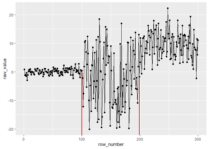
cpt_detect() dispatches to any supported method by
name:
cpt_detect(x, method = "binseg", change_in = "mean")
#> ggcpt (changepoint detection result)
#>   Method:          binseg
#>   Change in:       mean
#>   Changepoints found: 1
#>   CP convention:   left
#>   Penalty:         MBIC = NA
#>   Series length:   200
#>
#> Changepoints:
#> # A tibble: 1 × 2
#>      cp cp_value
#>   <dbl>    <dbl>
#> 1   100    0.467
cpt_detect(x, method = "wbs", change_in = "mean")
#> ggcpt (changepoint detection result)
#>   Method:          wbs
#>   Change in:       mean
#>   Changepoints found: 1
#>   CP convention:   left
#>   Penalty:         sSIC = NA
#>   Series length:   200
#>
#> Changepoints:
#> # A tibble: 1 × 2
#>      cp cp_value
#>   <int>    <dbl>
#> 1   100    0.467
cpt_detect(x, method = "fpop", change_in = "mean")
#> ggcpt (changepoint detection result)
#>   Method:          fpop
#>   Change in:       mean
#>   Changepoints found: 1
#>   CP convention:   left
#>   Penalty:         Manual = 10.5966347330961
#>   Series length:   200
#>
#> Changepoints:
#> # A tibble: 1 × 2
#>      cp cp_value
#>   <int>    <dbl>
#> 1   100    0.467
Use cpt_methods() to see all available and planned
methods with their engine packages and installation status:
cpt_methods()
#> # A tibble: 26 × 6
#>    method   change_in          engine         status    target_release installed
#>    <chr>    <chr>              <chr>          <chr>     <chr>          <lgl>
#>  1 pelt     mean, var, meanvar changepoint    available <NA>           TRUE
#>  2 binseg   mean, var, meanvar changepoint    available <NA>           TRUE
#>  3 segneigh mean, var, meanvar changepoint    available <NA>           TRUE
#>  4 amoc     mean, var, meanvar changepoint    available <NA>           TRUE
#>  5 np       distribution       changepoint.np available <NA>           TRUE
#>  6 ecp      distribution       ecp            available <NA>           TRUE
#>  7 fpop     mean               fpop           available <NA>           TRUE
#>  8 wbs      mean               wbs            available <NA>           TRUE
#>  9 wbs2     mean               breakfast      available <NA>           TRUE
#> 10 not      mean, var, slope   not            available <NA>           TRUE
#> # ℹ 16 more rowsggcpt_compare(x, methods = c("pelt", "binseg", "fpop", "wbs"))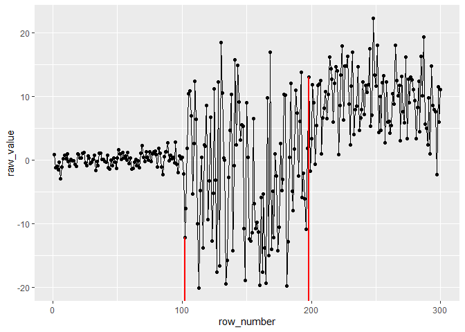
For a numeric summary, use ggcpt_compare_table():
ggcpt_compare_table(x, methods = c("pelt", "binseg", "fpop", "wbs"))
#> # A tibble: 4 × 3
#>   method    cp cp_value
#>   <chr>  <dbl>    <dbl>
#> 1 pelt     100    0.467
#> 2 binseg   100    0.467
#> 3 fpop     100    0.467
#> 4 wbs 100 0.467When ground truth changepoints are known, compute accuracy metrics:
cpt_metrics(pred = c(100), truth = c(100), n = 200)
#> # A tibble: 1 × 12
#>       n n_pred n_truth precision recall    f1 covering hausdorff rand_index
#>   <int>  <int>   <int>     <dbl>  <dbl> <dbl>    <dbl>     <dbl>      <dbl>
#> 1   200      1       1         1      1     1        1         0          1
#> # ℹ 3 more variables: annotation_error <int>, mae_matched <dbl>,
#> # rmse_matched <dbl>dat <- cpt_simulate(200, changepoints = c(100), change_in = "mean",
params = c(0, 10), sd = 1)
attributes(dat)$true_changepoints
#> [1] 100An alias rcpt() is provided for compatibility. Built-in
test signals include signal_blocks(),
signal_fms(), signal_mix(),
signal_teeth(), and signal_stairs().
Use cpt_penalty() to construct penalty values for use
with detection methods:
cpt_penalty("BIC", n = 200)
#> [1] 5.298317
cpt_penalty("AIC", n = 200)
#> [1] 2
cpt_penalty("Manual", value = 10)
#> [1] 10For fine-grained control, each detection engine has its own wrapper
that returns a ggcpt object directly:
fpop_wrapper(x, penalty = 2 * log(200))
#> ggcpt (changepoint detection result)
#>   Method:          fpop
#>   Change in:       mean
#>   Changepoints found: 1
#>   CP convention:   left
#>   Penalty:         Manual = 10.5966347330961
#>   Series length:   200
#>
#> Changepoints:
#> # A tibble: 1 × 2
#>      cp cp_value
#>   <int>    <dbl>
#> 1   100    0.467
wbs_wrapper(x, n_intervals = 2000)
#> ggcpt (changepoint detection result)
#>   Method:          wbs
#>   Change in:       mean
#>   Changepoints found: 1
#>   CP convention:   left
#>   Penalty:         sSIC = NA
#>   Series length:   200
#>
#> Changepoints:
#> # A tibble: 1 × 2
#>      cp cp_value
#>   <int>    <dbl>
#> 1   100    0.467
wbs2_wrapper(x)
#> ggcpt (changepoint detection result)
#>   Method:          wbs2
#>   Change in:       mean
#>   Changepoints found: 1
#>   CP convention:   left
#>   Penalty:         SDLL = NA
#>   Series length:   200
#>
#> Changepoints:
#> # A tibble: 1 × 2
#>      cp cp_value
#>   <int>    <dbl>
#> 1   100    0.467
not_wrapper(x, contrast = "pcwsConstMean")
#> ggcpt (changepoint detection result)
#>   Method:          not
#>   Change in:       mean
#>   Changepoints found: 1
#>   CP convention:   left
#>   Penalty:         sSIC = NA
#>   Series length:   200
#>
#> Changepoints:
#> # A tibble: 1 × 2
#>      cp cp_value
#>   <int>    <dbl>
#> 1   100    0.467
mosum_wrapper(x)
#> ggcpt (changepoint detection result)
#>   Method:          mosum
#>   Change in:       mean
#>   Changepoints found: 1
#>   CP convention:   left
#>   Penalty:         threshold = critical.value
#>   Series length:   200
#>
#> Changepoints:
#> # A tibble: 1 × 2
#>      cp cp_value
#>   <int>    <dbl>
#> 1   100    0.467
idetect_wrapper(x)
#> ggcpt (changepoint detection result)
#>   Method:          IDetect
#>   Change in:       mean
#>   Changepoints found: 1
#>   CP convention:   left
#>   Penalty:         threshold = NA
#>   Series length:   200
#>
#> Changepoints:
#> # A tibble: 1 × 2
#>      cp cp_value
#>   <int>    <dbl>
#> 1   100    0.467
tguh_wrapper(x)
#> ggcpt (changepoint detection result)
#>   Method:          tguh
#>   Change in:       mean
#>   Changepoints found: 1
#>   CP convention:   left
#>   Penalty:         threshold = NA
#>   Series length:   200
#>
#> Changepoints:
#> # A tibble: 1 × 2
#>      cp cp_value
#>   <int>    <dbl>
#> 1 100 0.467The package provides composable ggplot2 layers for changepoint visualisation:
library(ggplot2)

# Use geom_changepoint as a standalone layer
cp_tbl <- tidy(cpt_detect(x, method = "pelt", change_in = "mean"))
ggplot(data.frame(index = seq_along(x), value = x), aes(index, value)) +
  geom_line() +
  geom_changepoint(data = cp_tbl, aes(xintercept = cp), color = "red") +
  theme_ggcpt()

# Use stat_changepoint to compute and draw changepoints in one step
ggplot(data.frame(index = seq_along(x), value = x), aes(index, value)) +
  geom_line() +
  stat_changepoint(method = "pelt", color = "red")

# Shade alternating segments between changepoints
ggplot(data.frame(index = seq_along(x), value = x), aes(index, value)) +
  geom_line() +
  annotate_segments(cp = cp_tbl$cp, n = length(x))

# Highlight segments with geom_cpt_segment
ggplot(data.frame(index = seq_along(x), value = x), aes(index, value)) +
  geom_line() +
  geom_cpt_segment(data = cp_tbl, aes(xintercept = cp), color = "blue")

# Draw confidence intervals with geom_cpt_ci (when the engine provides them)
ggplot(data.frame(index = seq_along(x), value = x), aes(index, value)) +
  geom_line() +
geom_cpt_ci(data = cp_tbl, aes(xintercept = cp, ymin = lower, ymax = upper))When multiple annotation sets are available, use
cpt_metrics_annotated() and visualise with
ggcpt_eval():
cpt_metrics_annotated(c(100), list(c(100), c(101), c(99)), n = 200, margin = 5)
#> # A tibble: 1 × 7
#>       n n_annotators n_pred precision recall    f1 covering
#>   <dbl>        <int>  <int>     <dbl>  <dbl> <dbl>    <dbl>
#> 1 200 3 1 1 1 1 0.993Advanced users can construct ggcpt objects directly or
test for the class:
new_ggcpt(
  changepoints = tibble::tibble(cp = 100L, cp_value = 5.0),
  data = tibble::tibble(index = 1:200, value = rnorm(200)),
  method = "manual"
)
is_ggcpt(x)The ecp_wrapper() and its plotting function
ggecpplot() provide direct access to the ecp engine:
ecp_wrapper(x, algorithm = "divisive")
ggecpplot(x, algorithm = "divisive")The original cpt_wrapper(), ecp_wrapper(),
ggcptplot(), and ggecpplot() continue to work
unchanged for backward compatibility.
cpt_wrapper(x)
#> # A tibble: 1 × 2
#>      cp cp_value
#>   <int>    <dbl>
#> 1   100    0.467
ggcptplot(x)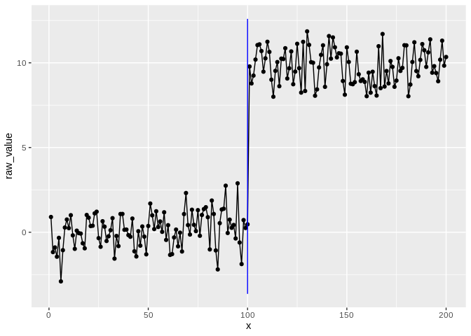
The ggcpt class also provides:
res <- cpt_detect(x, method = "pelt", change_in = "mean")
summary(res)          # human-readable digest
#> ggcpt Summary
#>   Method:                   pelt
#>   Change in:                mean
#>   Changepoints found:       1
#>   CP convention:            left
#>   Series length:            200
#>   Penalty:                  MBIC = NA
#>   Runtime (seconds):        0.006
#>
#> Segments:
#> # A tibble: 2 × 5
#>   seg_id start   end     n param_estimate
#>    <int> <dbl> <int> <dbl>          <dbl>
#> 1      1     1   100   100          0.139
#> 2      2   101   200   100          9.80
#>
#> Changepoints:
#> # A tibble: 1 × 2
#>      cp cp_value
#>   <int>    <dbl>
#> 1   100    0.467
as_tibble(res)        # tibble of changepoints
#> # A tibble: 1 × 2
#>      cp cp_value
#>   <int>    <dbl>
#> 1   100    0.467
as.data.frame(res)    # data frame of changepoints
#>    cp cp_value
#> 1 100 0.467023
format(res)           # one-line summary string
#> [1] "ggcpt [pelt] 1 changepoint(s) on 200 observations"
plot(res)             # base-graphics fallback (delegates to autoplot)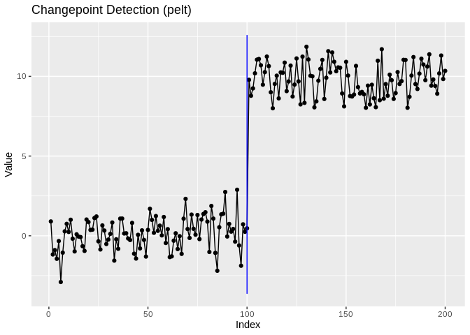
See the vignettes for a comprehensive walkthrough:
vignette("ggchangepoint", package = "ggchangepoint") —
feature tourvignette("introduction", package = "ggchangepoint")vignette("comparison", package = "ggchangepoint")These binaries (installable software) and packages are in development.
They may not be fully stable and should be used with caution. We make no claims about them.
Health stats visible at Monitor.