The hardware and bandwidth for this mirror is donated by dogado GmbH, the Webhosting and Full Service-Cloud Provider. Check out our Wordpress Tutorial.
If you wish to report a bug, or if you are interested in having us mirror your free-software or open-source project, please feel free to contact us at mirror[@]dogado.de.

ggDoE

Installation

You can install:

• the latest release from CRAN with

install.packages('ggDoE')

• the development version from GitHub with

if (!require("pak")) install.packages("pak")
pak::pak("toledo60/ggDoE")

Overview

With ggDoE you’ll be able to generate common plots used in Design of Experiments with ggplot2.

library(ggDoE)

The following plots are currently available:

1. Alias Matrix
2. Box-Cox Transformation
3. Lambda Plot
4. Boxplots
5. Regression Diagnostic Plots
6. Half-Normal Plot
7. Interaction Effects Plot for a Factorial Design
8. Main Effects Plot for a Factorial Design
9. Contour Plots for Response Surface Methodology
10. Pareto Plot
11. Two Dimensional Projections of a Latin Hypercube Design

The following datasets/designs are included in ggDoE as tibbles:

• adapted_epitaxial: Adapted epitaxial layer experiment obtain from the book
  “Experiments: Planning, Analysis, and Optimization, 2nd Edition”

• original_epitaxial: Original epitaxial layer experiment obtain from the book
  “Experiments: Planning, Analysis, and Optimization, 2nd Edition”

• pulp_experiment: Reflectance Data, Pulp Experiment obtain from the book
  “Experiments: Planning, Analysis, and Optimization, 2nd Edition”

• girder_experiment: Girder experiment obtain from the book
  “Experiments: Planning, Analysis, and Optimization, 2nd Edition”

• aliased_design: D-efficient minimal aliasing design obtained from the article
  “Efficient Designs With Minimal Aliasing by Bradley Jones and Christopher J. Nachtsheim”

Citation

If you want to cite this package in a scientific journal or in any other context, run the following code in your R console

citation('ggDoE')

Warning in citation("ggDoE"): could not determine year for 'ggDoE' from package
DESCRIPTION file

To cite package 'ggDoE' in publications use:

  Toledo Luna J (????). _ggDoE: Modern Graphs for Design of Experiments
  with 'ggplot2'_. R package version 0.8, <https://ggdoe.netlify.app>.

A BibTeX entry for LaTeX users is

  @Manual{,
    title = {ggDoE: Modern Graphs for Design of Experiments with 'ggplot2'},
    author = {Jose {Toledo Luna}},
    note = {R package version 0.8},
    url = {https://ggdoe.netlify.app},
  }

Contributing to the package

I welcome feedback, suggestions, issues, and contributions! Check out the CONTRIBUTING file for more details.

Examples of Plots

Alias Matrix

Correlation matrix plot to visualize the Alias matrix

alias_matrix(design=aliased_design)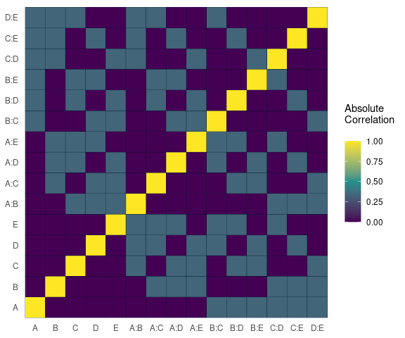

Box-Cox Transformation

model <- lm(s2 ~ (A+B+C+D),data = adapted_epitaxial)
boxcox_transform(model,lambda = seq(-5,5,0.2))

Lambda Plot

Obtain the trace plot of the t-statistics after applying Boxcox transformation across a specified sequence of lambda values

model <-  lm(s2 ~ (A+B+C)^2,data=original_epitaxial)
lambda_plot(model)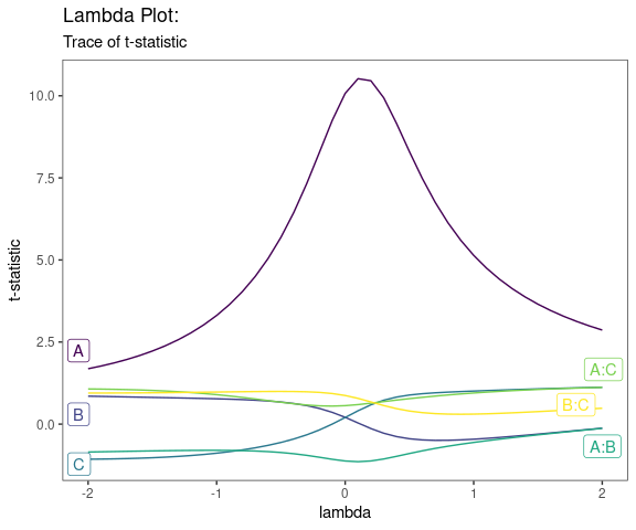

lambda_plot(model, lambda = seq(0,2,by=0.1))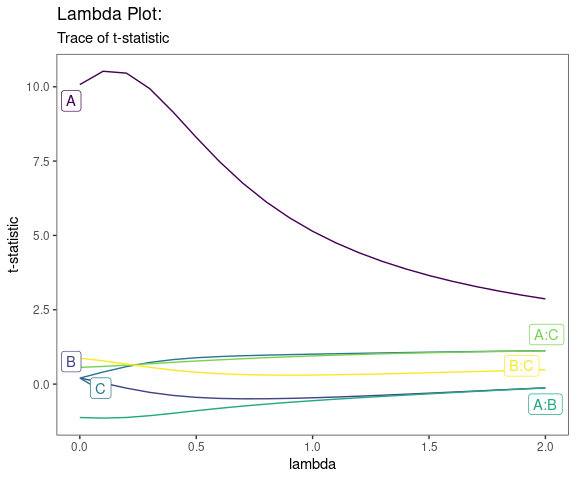

Boxplots

data <- ToothGrowth
data$dose <- factor(data$dose,levels = c(0.5, 1, 2),
                    labels = c("D0.5", "D1", "D2"))

gg_boxplots(data,y = 'len',x = 'dose')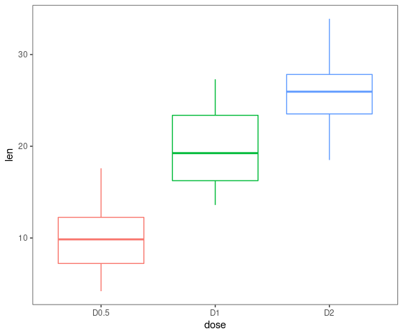

gg_boxplots(data,y = 'len',x = 'dose',
            group_var = 'supp',
            color_palette = 'viridis',
            jitter_points = TRUE)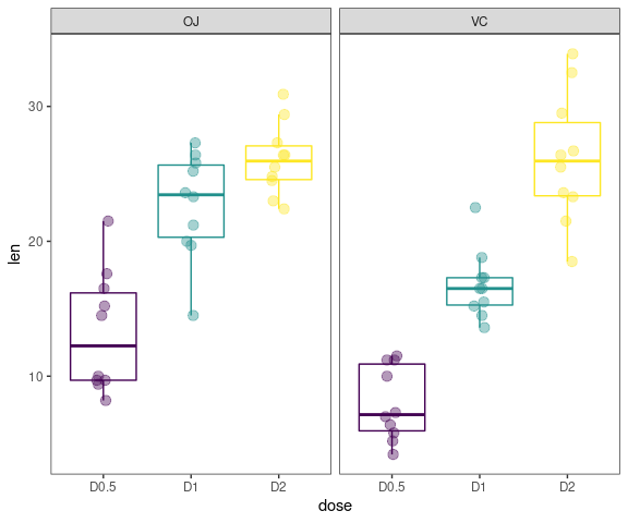

Regression Diagnostic Plots

1. Residual vs. Fitted Values
2. Normal-QQ plot
3. Scale-Location plot
4. Residual vs. Leverage
5. Cook’s Distance
6. Collinearity

The default plots are 1-4

model <- lm(mpg ~ wt + am + gear + vs * cyl, data = mtcars)
gg_lm(model,which_plots=1:6)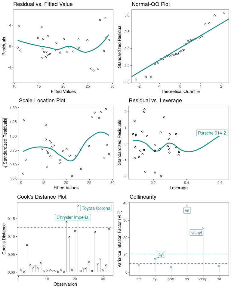

Half-Normal Plot

model <- lm(ybar ~ (A+B+C+D)^4,data=adapted_epitaxial)
half_normal(model)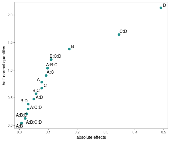

half_normal(model,method='Zahn',alpha=0.1,
            ref_line=TRUE,label_active=TRUE,
            margin_errors=TRUE)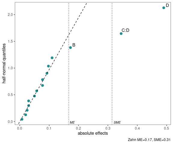

Interaction Effects Plot

Interaction effects plot between two factors in a factorial design

interaction_effects(adapted_epitaxial,response = 'ybar',
                    exclude_vars = c('s2','lns2'))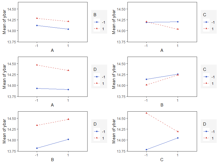

interaction_effects(adapted_epitaxial,response = 'ybar',
                    exclude_vars = c('A','s2','lns2'),
                    n_columns=3)

Main Effects Plots

Main effect plots for each factor in a factorial design

main_effects(original_epitaxial,
             response='s2',
             exclude_vars = c('A','ybar','lns2'),
             color_palette = 'viridis',
             n_columns=3)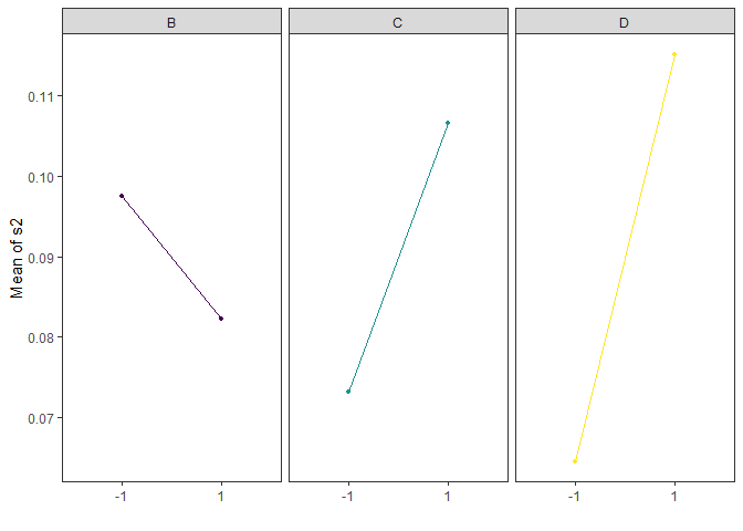

Contour Plots

contour plot(s) that display the fitted surface for an rsm object involving two or more numerical predictors

heli.rsm <- rsm::rsm(ave ~ SO(x1, x2, x3, x4), 
                     data = rsm::heli)

gg_rsm(heli.rsm,formula = ~x1+x2+x3+x4,
       at = rsm::xs(heli.rsm))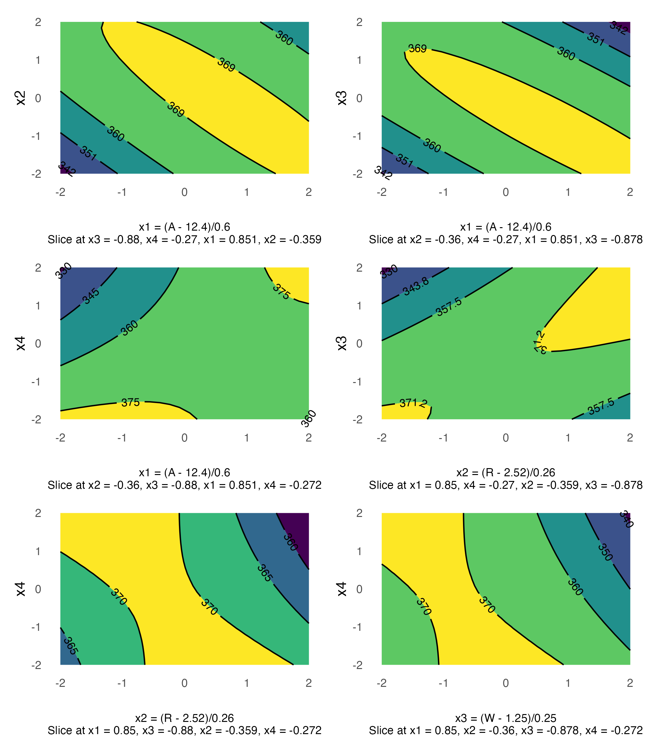

Pareto Plot

Pareto plot of effects with cutoff values for the margin of error (ME) and simultaneous margin of error (SME)

model <- lm(lns2 ~ (A+B+C+D)^4,data=original_epitaxial)
pareto_plot(model)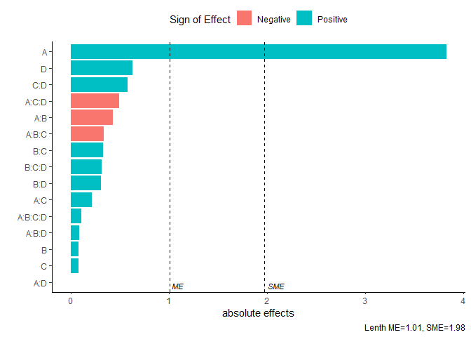

pareto_plot(model,method='Zahn',alpha=0.1)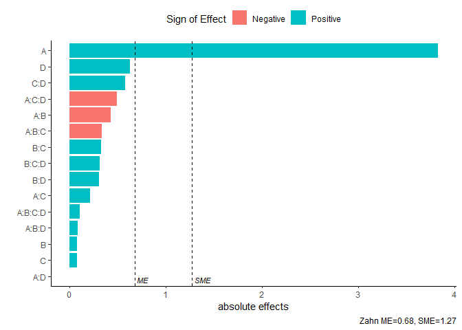

Two Dimensional Projections

This function will output all two dimensional projections from a Latin hypercube design

set.seed(10)
X <- lhs::randomLHS(n=10, k=4)
pair_plots(X,n_columns=3,grid = TRUE)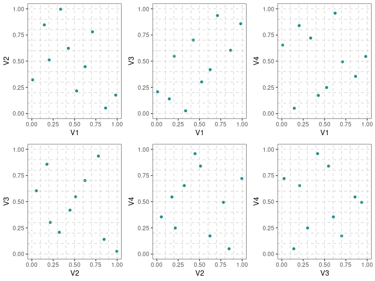

These binaries (installable software) and packages are in development.
They may not be fully stable and should be used with caution. We make no claims about them.
Health stats visible at Monitor.