The hardware and bandwidth for this mirror is donated by dogado GmbH, the Webhosting and Full Service-Cloud Provider. Check out our Wordpress Tutorial.
If you wish to report a bug, or if you are interested in having us mirror your free-software or open-source project, please feel free to contact us at mirror[@]dogado.de.

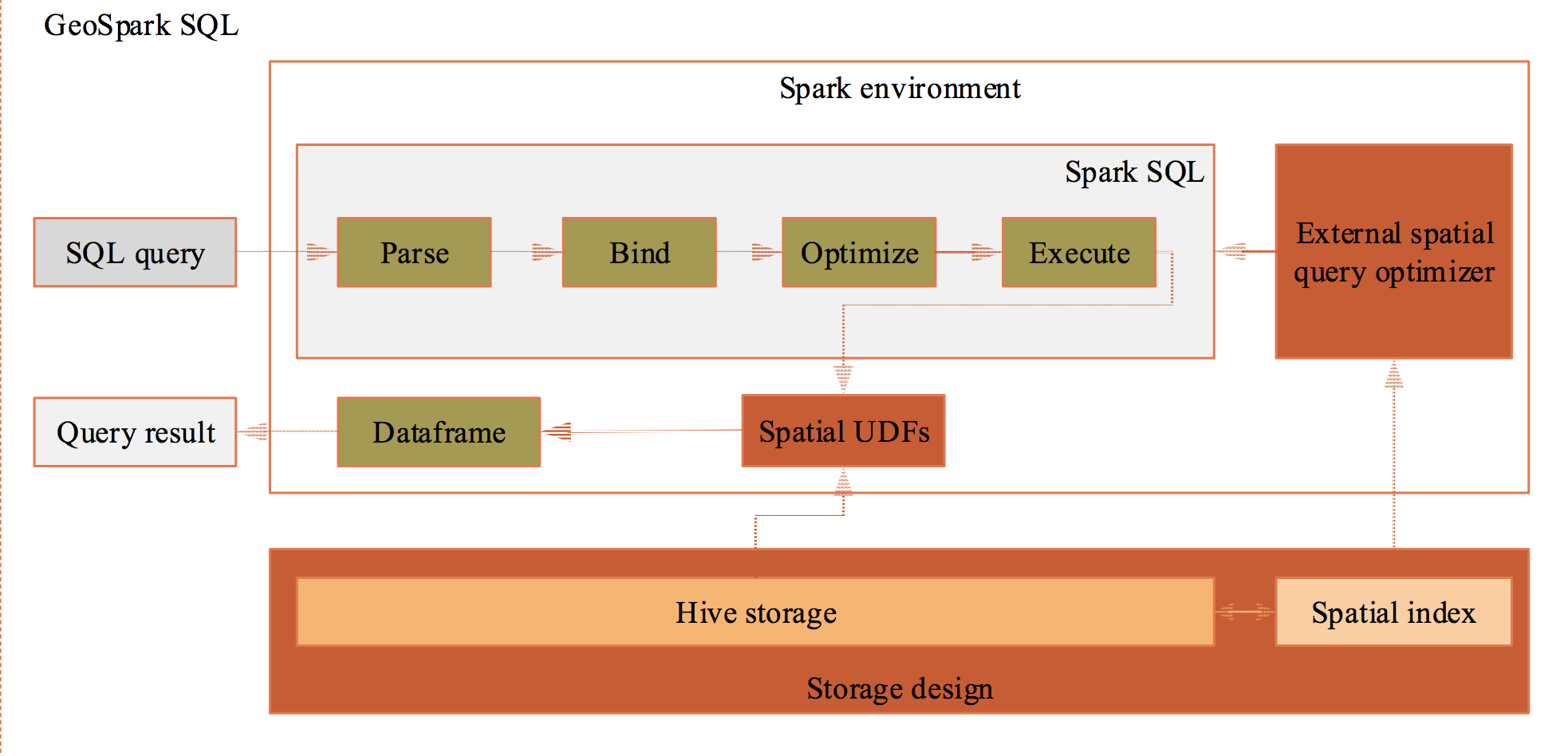
Goal: make traditional GISer handle geospatial big data easier.
The origin idea comes from Uber, which proposed a ESRI Hive UDF + Presto solution to solve large-scale geospatial data processing problem with spatial index in production.
However, The Uber solution is not open source yet and Presto is not popular than Spark.
In that, geospark R package aims at bringing local sf functions to distributed
spark mode with GeoSpark scala
package.
Currently, geospark support the most of important
sf functions in spark, here is a summary
comparison. And the geospark R package is keeping close
with geospatial and big data community, which powered by sparklyr, sf, dplyr and dbplyr.
This package requires Apache Spark 2.X which you can install using
sparklyr::install_spark("2.3"), and spark2.4 is not
supported yet; in addition, you can install geospark as
follows:
pak::pkg_install("harryprince/geospark")In this example we will join spatial data using quadrad tree
indexing. First, we will initialize the geospark extension
and connect to Spark using sparklyr:
library(sparklyr)
library(geospark)

sc <- spark_connect(master = "local")
register_gis(sc)
Next we will load some spatial dataset containing as polygons and points.
polygons <- read.table(system.file(package="geospark","examples/polygons.txt"), sep="|", col.names=c("area","geom"))
points <- read.table(system.file(package="geospark","examples/points.txt"), sep="|", col.names=c("city","state","geom"))

polygons_wkt <- copy_to(sc, polygons)
points_wkt <- copy_to(sc, points)
And we can quickly visulize the dataset by mapview and
sf.
M1 = polygons %>%
sf::st_as_sf(wkt="geom") %>% mapview::mapview()


M2 = points %>%
sf::st_as_sf(wkt="geom") %>% mapview::mapview()

M1+M2Now we can perform a GeoSpatial join using the
st_contains which converts wkt into geometry
object. To get the original data from wkt format, we will
use the st_geomfromwkt functions. We can execute this
spatial query using DBI:
DBI::dbGetQuery(sc, "
  SELECT area, state, count(*) cnt FROM
    (SELECT area, ST_GeomFromWKT(polygons.geom) as y FROM polygons) polygons
  INNER JOIN
    (SELECT ST_GeomFromWKT (points.geom) as x, state, city FROM points) points
  WHERE ST_Contains(polygons.y,points.x) GROUP BY area, state")
area state cnt
1 texas area TX 10
2 dakota area SD 1
3 dakota area ND 10
4 california area CA 10
5 new york area NY 9You can also perform this query using dplyr as
follows:
library(dplyr)
polygons_wkt <- mutate(polygons_wkt, y = st_geomfromwkt(geom))
points_wkt <- mutate(points_wkt, x = st_geomfromwkt(geom))

sc_res <- inner_join(polygons_wkt,
                     points_wkt,
                     sql_on = sql("st_contains(y,x)")) %>%
  group_by(area, state) %>%
  summarise(cnt = n())

sc_res %>%
  head()
# Source: spark<?> [?? x 3]
# Groups: area
area state cnt
<chr> <chr> <dbl>
1 texas area TX 10
2 dakota area SD 1
3 dakota area ND 10
4 california area CA 10
5 new york area NY 9The final result can be present by leaflet.
Idx_df = collect(sc_res) %>%
right_join(polygons,by = (c("area"="area"))) %>%
sf::st_as_sf(wkt="geom")

Idx_df %>%
leaflet::leaflet() %>%
leaflet::addTiles() %>%
leaflet::addPolygons(popup = ~as.character(cnt),color=~colormap::colormap_pal()(cnt))
Finally, we can disconnect:
spark_disconnect_all()To improve performance, it is recommended to use the
KryoSerializer and the GeoSparkKryoRegistrator
before connecting as follows:
conf <- spark_config()
conf$spark.serializer <- "org.apache.spark.serializer.KryoSerializer"
conf$spark.kryo.registrator <- "org.datasyslab.geospark.serde.GeoSparkKryoRegistrator"This performance comparison is an extract from the original GeoSpark: A Cluster Computing Framework for Processing Spatial Data paper:
| No. | test case | the number of records |
|---|---|---|
| 1 | SELECT IDCODE FROM zhenlongxiang WHERE ST_Disjoint(geom,ST_GeomFromText(‘POLYGON((517000 1520000,619000 1520000,619000 2530000,517000 2530000,517000 1520000))’)); | 85,236 rows |
| 2 | SELECT fid FROM cyclonepoint WHERE ST_Disjoint(geom,ST_GeomFromText(‘POLYGON((90 3,170 3,170 55,90 55,90 3))’,4326)) | 60,591 rows |
Query performance(ms),
| No. | PostGIS/PostgreSQL | GeoSpark SQL | ESRI Spatial Framework for Hadoop |
|---|---|---|---|
| 1 | 9631 | 480 | 40,784 |
| 2 | 110872 | 394 | 64,217 |
According to this paper, the Geospark SQL definitely outperforms PG and ESRI UDF under a very large data set.
If you are wondering how the spatial index accelerate the query process, here is a good Uber example: Unwinding Uber’s Most Efficient Service and the Chinese translation version
| name | desc |
|---|---|
ST_GeomFromWKT |
Construct a Geometry from Wkt. |
ST_GeomFromWKB |
Construct a Geometry from Wkb. |
ST_GeomFromGeoJSON |
Construct a Geometry from GeoJSON. |
ST_Point |
Construct a Point from X and Y. |
ST_PointFromText |
Construct a Point from Text, delimited by Delimiter. |
ST_PolygonFromText |
Construct a Polygon from Text, delimited by Delimiter. |
ST_LineStringFromText |
Construct a LineString from Text, delimited by Delimiter. |
ST_PolygonFromEnvelope |
Construct a Polygon from MinX, MinY, MaxX, MaxY. |
| name | desc |
|---|---|
ST_Length |
Return the perimeter of A |
ST_Area |
Return the area of A |
ST_Distance |
Return the Euclidean distance between A and B |
| name | desc |
|---|---|
ST_Contains |
|
ST_Intersects |
|
ST_Within |
|
ST_Equals |
|
ST_Crosses |
|
ST_Touches |
|
ST_Overlaps |
ST_Distance:
Spark GIS SQL mode example:
SELECT *
FROM pointdf1, pointdf2
WHERE ST_Distance(pointdf1.pointshape1,pointdf2.pointshape2) <= 2
Tidyverse style example:
st_join(x = pointdf1,
           y = pointdf2,
join = sql("ST_Distance(pointshape1, pointshape2) <= 2"))| name | desc |
|---|---|
ST_Envelope_Aggr |
Return the entire envelope boundary of all geometries in A |
ST_Union_Aggr |
Return the polygon union of all polygons in A |
| name | desc |
|---|---|
ST_ConvexHull |
Return the Convex Hull of polgyon A |
ST_Envelope |
Return the envelop boundary of A |
ST_Centroid |
Return the centroid point of A |
ST_Transform |
Transform the Spatial Reference System / Coordinate Reference System of A, from SourceCRS to TargetCRS |
ST_IsValid |
Test if a geometry is well formed |
ST_PrecisionReduce |
Reduce the decimals places in the coordinates of the geometry to the given number of decimal places. The last decimal place will be rounded. |
ST_IsSimple |
Test if geometry’s only self-intersections are at boundary points. |
ST_Buffer |
Returns a geometry/geography that represents all points whose distance from this Geometry/geography is less than or equal to distance. |
ST_AsText |
Return the Well-Known Text string representation of a geometry |
These binaries (installable software) and packages are in development.
They may not be fully stable and should be used with caution. We make no claims about them.
Health stats visible at Monitor.