The hardware and bandwidth for this mirror is donated by dogado GmbH, the Webhosting and Full Service-Cloud Provider. Check out our Wordpress Tutorial.
If you wish to report a bug, or if you are interested in having us mirror your free-software or open-source project, please feel free to contact us at mirror[@]dogado.de.
The goal of geos is to provide access to the GEOS C API by vectorizing the C functions for use in R. See the package function reference for which functions are implemented in the R API.
You can install the released version of geos from CRAN with:
install.packages("geos")And the development version from GitHub with:
# install.packages("remotes")
remotes::install_github("paleolimbot/geos")
If you can load the package, you’re good to go!
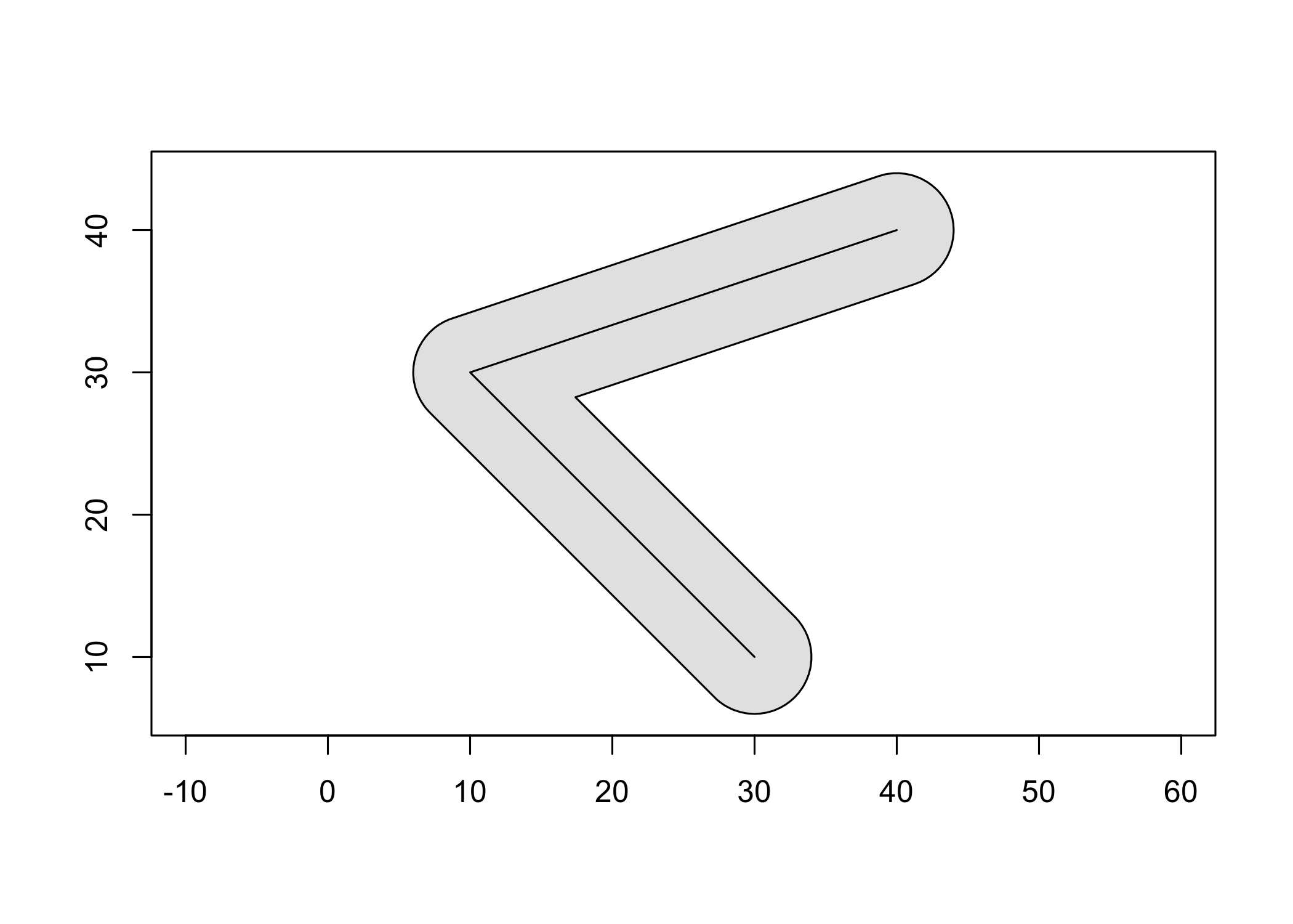
library(geos)Buffer a line and plot it!
line <- as_geos_geometry("LINESTRING (30 10, 10 30, 40 40)")
plot(geos_buffer(line, distance = 4), col = "grey90")
plot(line, add = T)
The geos package is designed to work with dplyr package, so you can work with geometry vectors as a data frame column:
library(dplyr)
#>
#> Attaching package: 'dplyr'
#> The following objects are masked from 'package:stats':
#>
#>     filter, lag
#> The following objects are masked from 'package:base':
#>
#>     intersect, setdiff, setequal, union

# map data from the maps package via ggplot2
states_df <- as_tibble(ggplot2::map_data("state"))
states_df
#> # A tibble: 15,537 × 6
#>     long   lat group order region  subregion
#>    <dbl> <dbl> <dbl> <int> <chr>   <chr>
#>  1 -87.5  30.4     1     1 alabama <NA>
#>  2 -87.5  30.4     1     2 alabama <NA>
#>  3 -87.5  30.4     1     3 alabama <NA>
#>  4 -87.5  30.3     1     4 alabama <NA>
#>  5 -87.6  30.3     1     5 alabama <NA>
#>  6 -87.6  30.3     1     6 alabama <NA>
#>  7 -87.6  30.3     1     7 alabama <NA>
#>  8 -87.6  30.3     1     8 alabama <NA>
#>  9 -87.7  30.3     1     9 alabama <NA>
#> 10 -87.8  30.3     1    10 alabama <NA>
#> # … with 15,527 more rows

states_df %>%
  group_by(region, group) %>%
  summarise(geometry = geos_make_polygon(long, lat)) %>%
  summarise(geometry = geos_make_collection(geometry, "multipolygon"))
#> `summarise()` has grouped output by 'region'. You can override using the
#> `.groups` argument.
#> # A tibble: 49 × 2
#>    region               geometry
#>    <chr>                <geos_geom>
#>  1 alabama              <MULTIPOLYGON [-88.476 30.241...-84.901 35.013]>
#>  2 arizona              <MULTIPOLYGON [-114.809 31.347...-109.040 37.002]>
#>  3 arkansas             <MULTIPOLYGON [-94.624 32.997...-89.651 36.509]>
#>  4 california           <MULTIPOLYGON [-124.383 32.538...-114.133 42.021]>
#>  5 colorado             <MULTIPOLYGON [-109.063 36.984...-102.044 41.018]>
#>  6 connecticut          <MULTIPOLYGON [-73.722 41.012...-71.780 42.049]>
#>  7 delaware             <MULTIPOLYGON [-75.802 38.457...-75.052 39.849]>
#>  8 district of columbia <MULTIPOLYGON [-77.137 38.806...-76.931 38.996]>
#>  9 florida              <MULTIPOLYGON [-87.640 25.130...-80.042 31.008]>
#> 10 georgia              <MULTIPOLYGON [-85.611 30.355...-80.844 34.996]>
#> # … with 39 more rows
The easiest way to get data into and out of the package is using the sf package.
library(sf)
#> Linking to GEOS 3.11.0, GDAL 3.5.1, PROJ 9.0.1; sf_use_s2() is TRUE
nc <- read_sf(system.file("shape/nc.shp", package = "sf")) %>%
  st_transform(32119) # North Carolina state plane, m.

nc_geos <- as_geos_geometry(nc)

nc_geos %>%
  geos_make_collection() %>%
  geos_unary_union() %>%
  st_as_sfc(nc_state)
#> Geometry set for 1 feature
#> Geometry type: MULTIPOLYGON
#> Dimension:     XY
#> Bounding box:  xmin: 123829 ymin: 14744.69 xmax: 930521.8 ymax: 318259.9
#> Projected CRS: NAD83 / North Carolina
#> MULTIPOLYGON (((138426 177699.3, 145548.6 17783...
These binaries (installable software) and packages are in development.
They may not be fully stable and should be used with caution. We make no claims about them.
Health stats visible at Monitor.