The hardware and bandwidth for this mirror is donated by dogado GmbH, the Webhosting and Full Service-Cloud Provider. Check out our Wordpress Tutorial.
If you wish to report a bug, or if you are interested in having us mirror your free-software or open-source project, please feel free to contact us at mirror[@]dogado.de.
This is a super simple package to help make scatter plots of two
variables after residualizing by covariates. This package uses
fixest so things are super fast. This is meant to (as much
as possible) be a drop in replacement for fixest::feols.
You should be able to replace feols with
fwl_plot and get a plot.
The stable version of fwlplot is available on CRAN.
install.packages("fwlplot")Or, you can grab the latest development version from GitHub.
# install.packages("remotes")
remotes::install_github("kylebutts/fwlplot")Here’s a simple example with fixed effects removed by
fixest.
library(fwlplot)
library(fixest)
flights <- data.table::fread("https://raw.githubusercontent.com/Rdatatable/data.table/master/vignettes/flights14.csv")
flights[, long_distance := distance > 2000]
# Sample 10000 rows
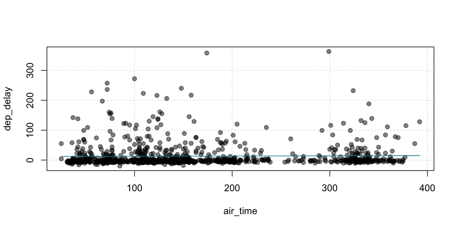
sample <- flights[sample(.N, 10000)]# Without covariates = scatterplot
fwl_plot(dep_delay ~ air_time, data = sample)
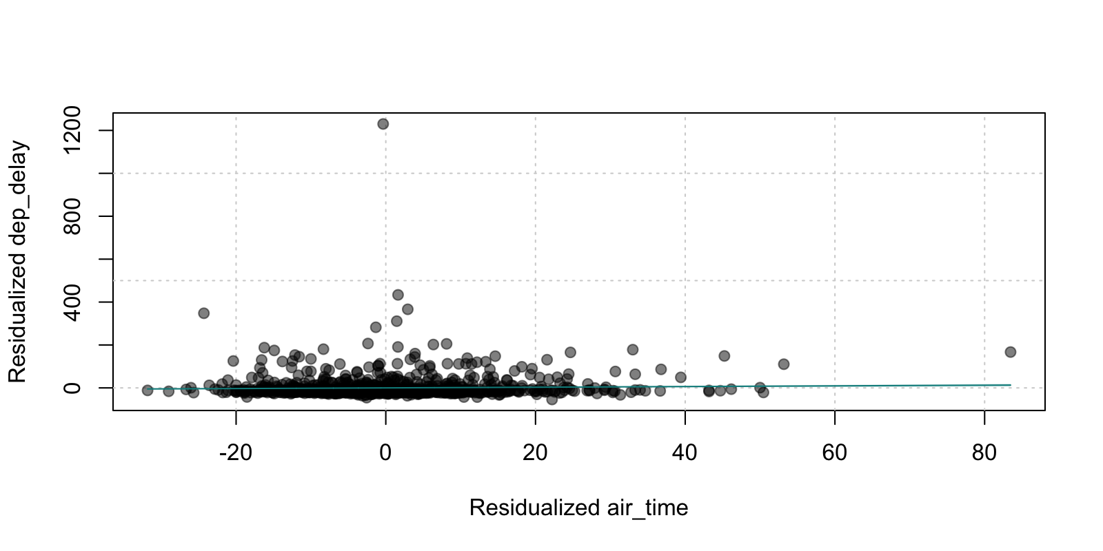
# With covariates = FWL'd scatterplot
fwl_plot(
  dep_delay ~ air_time | origin + dest,
  data = sample, vcov = "hc1"
)
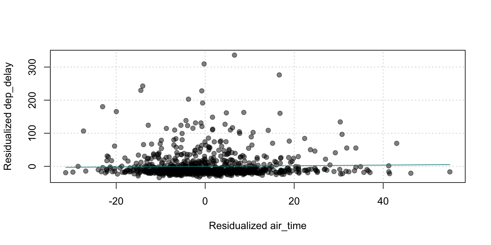
If you have a large dataset, we can plot a sample of points with the
n_sample argument. This determines the number of points
per plot (see multiple estimation below).
fwl_plot(
  dep_delay ~ air_time | origin + dest,
  # Full dataset for estimation, 1000 obs. for plotting
  data = flights, n_sample = 1000
)
feols
compatabilityThis is meant to be a 1:1 drop-in replacement with fixest, so
everything should work by just replacing feols with
feols(
  dep_delay ~ air_time | origin + dest,
  data = sample, subset = ~long_distance, cluster = ~origin
)
#> OLS estimation, Dep. Var.: dep_delay
#> Observations: 1,746
#> Subset: long_distance
#> Fixed-effects: origin: 2,  dest: 15
#> Standard-errors: Clustered (origin)
#>          Estimate Std. Error t value Pr(>|t|)
#> air_time 0.081485   0.052053 1.56541   0.3619
#> ---
#> Signif. codes:  0 '***' 0.001 '**' 0.01 '*' 0.05 '.' 0.1 ' ' 1
#> RMSE: 39.9     Adj. R2: 0.005478
#> Within R2: 0.001048fwl_plot(
dep_delay ~ air_time | origin + dest,
data = sample, subset = ~long_distance, cluster = ~origin
)
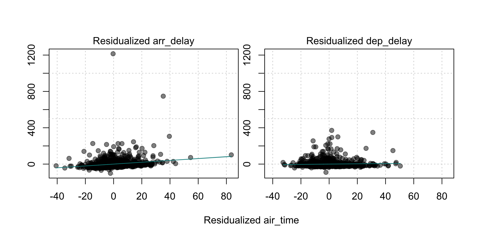
# Multiple y variables
fwl_plot(
  c(dep_delay, arr_delay) ~ air_time | origin + dest,
  data = sample
)
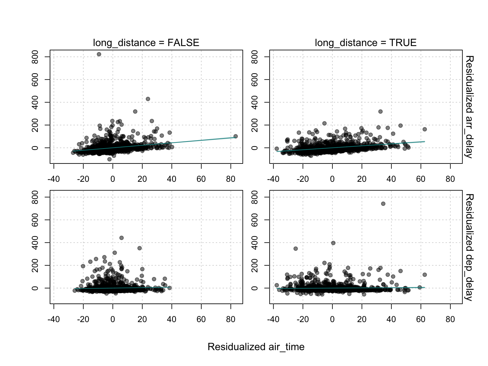
# `split` sample
fwl_plot(
  c(dep_delay, arr_delay) ~ air_time | origin + dest,
  data = sample, split = ~long_distance, n_sample = 1000
)
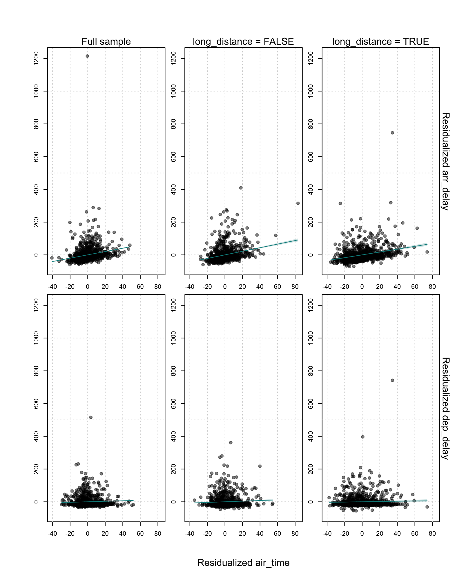
# `fsplit` = `split` sample and Full sample
fwl_plot(
  c(dep_delay, arr_delay) ~ air_time | origin + dest,
  data = sample, fsplit = ~long_distance, n_sample = 1000
)
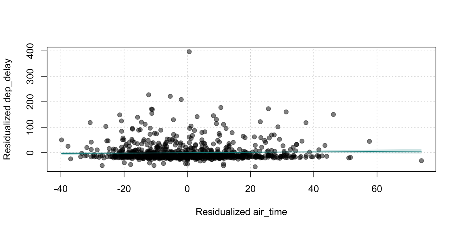
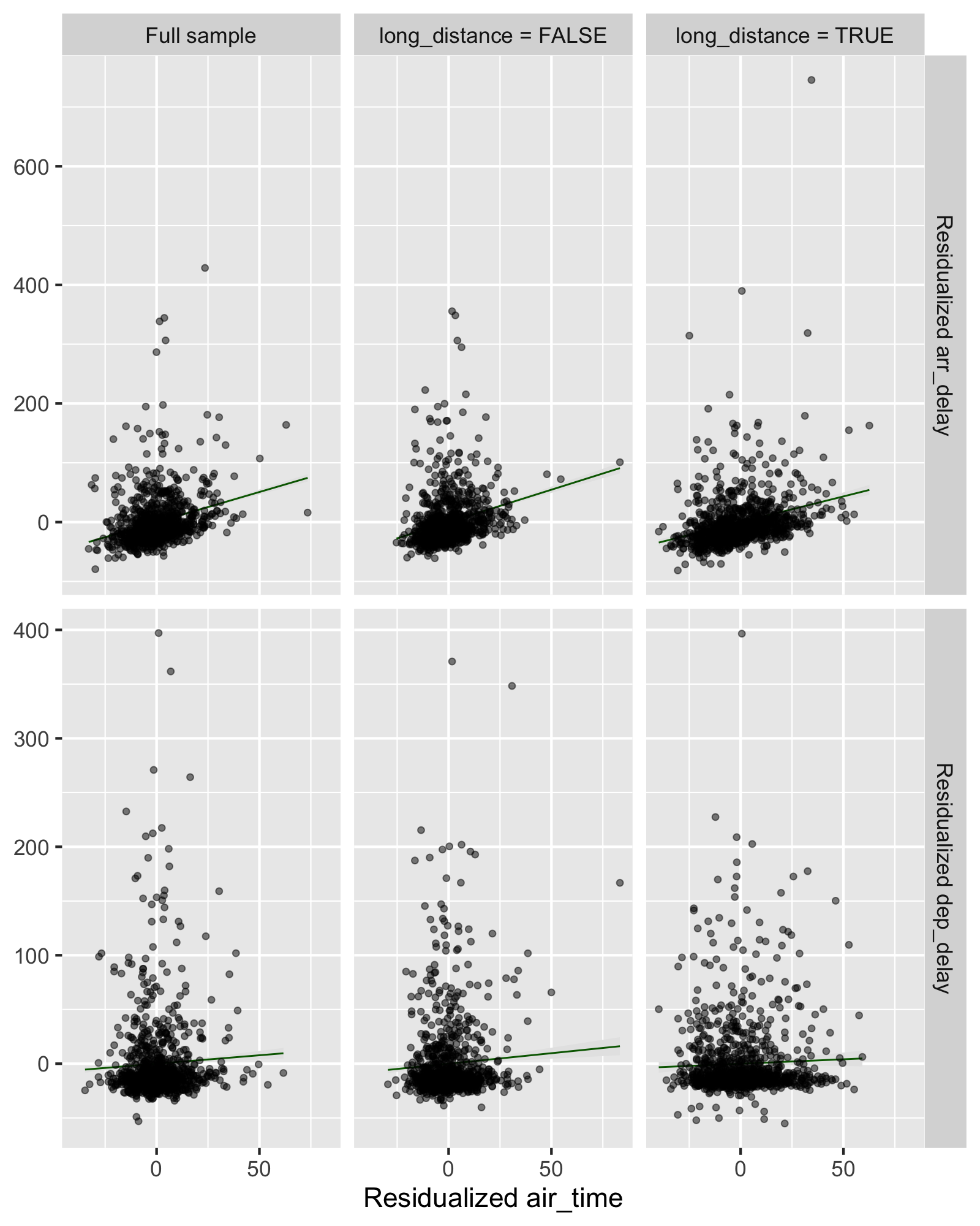
library(ggplot2)
theme_set(theme_grey(base_size = 16))
fwl_plot(
  c(dep_delay, arr_delay) ~ air_time | origin + dest,
  data = sample, fsplit = ~long_distance,
  n_sample = 1000, ggplot = TRUE
)
These binaries (installable software) and packages are in development.
They may not be fully stable and should be used with caution. We make no claims about them.
Health stats visible at Monitor.