The hardware and bandwidth for this mirror is donated by dogado GmbH, the Webhosting and Full Service-Cloud Provider. Check out our Wordpress Tutorial.
If you wish to report a bug, or if you are interested in having us mirror your free-software or open-source project, please feel free to contact us at mirror[@]dogado.de.
fwb: Fractional
Weighted Bootstrapfwb implements the fractional weighted bootstrap (FWB),
also known as the Bayesian bootstrap, following the treatment by Xu et
al. (2020). The FWB involves generating sets of weights from a uniform
Dirichlet distribution to be used in estimating statistics of interest,
which yields a posterior distribution that can be interpreted in the
same way the traditional (resampling-based) bootstrap distribution can
be. The primary function is fwb(), which is essentially a
drop-in for boot::boot() in that it takes in a dataset and
a function and applies that function to the dataset and a randomly
generated set of case weights. Also included are fwb.ci(),
a drop-in for boot::boot.ci() for computing various kinds
of confidence intervals (e.g., percentile, normal, bias-corrected
percentile, etc.), and vcovFWB(), a drop-in for
sandwich::vcovBS() for computing a coefficient covariance
matrix from a regression model using the FWB.
Check out the fwb website!
You can install the current stable version of fwb from
CRAN with:
install.packages("fwb")You can install the development version of fwb from GitHub with:
# install.packages("remotes")
remotes::install_github("ngreifer/fwb")Below are some examples of how to use fwb. We set a seed
to ensure all results are replicable. (Note that when parallel
processing is used, a special kind of seed needs to be set; see
vignette("fwb-rep") for details.)
library("fwb")
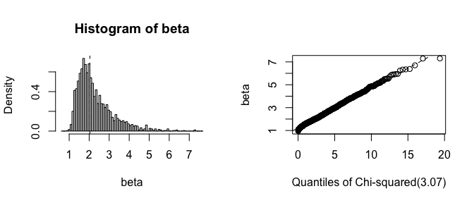
set.seed(123456, "L'Ecuyer-CMRG")This example involves performing a Weibull analysis to estimate the \(\beta\) (shape) parameter of the Weibull distribution characterizing the time to failure of a set of aircraft engines. Among the 1703 engines, there were only 6 failures and 1697 right-censored observations. The traditional (resampling-based) bootstrap would fail if a bootstrap replication omitted the 6 failures, but all failures are retained when using the FWB, which makes it particularly effective for this analysis.
data("bearingcage", package = "fwb")

# Function to compute the scale (eta) and shape (beta) parameters
# from weighted data
weibull_est <- function(data, w) {
  fit <- survival::survreg(survival::Surv(hours, failure) ~ 1,
                           data = data, weights = w,
                           dist = "weibull")

  c(eta = unname(exp(coef(fit))),
    beta = 1 / fit$scale)
}

# 1999 bootstrap replications; more is always better
fwb_est <- fwb(bearingcage, statistic = weibull_est,
               R = 1999, verbose = FALSE)
fwb_est
#> FRACTIONAL WEIGHTED BOOTSTRAP
#>
#> Call:
#> fwb(data = bearingcage, statistic = weibull_est, R = 1999, verbose = FALSE)
#>
#> Bootstrap Statistics :
#>          original         bias   std. error
#> eta  11792.178173 7722.5390790 2.652048e+04
#> beta     2.035319    0.2326988 8.790395e-01

# Bias-corrected accelerated percentile
# confidence interval
summary(fwb_est, ci.type = "bca")
#>      Estimate Std. Error CI 2.5 % CI 97.5 %
#> eta  1.18e+04   2.65e+04 3.15e+03  7.17e+04
#> beta 2.04e+00   8.79e-01 1.24e+00  4.55e+00

# Plot the bootstrap distribution
plot(fwb_est, index = "beta", qdist = "chisq")
infert datasetThis example demonstrates using vcovFWB() to estimate
standard errors for the effect of spontaneous and induced abortions on
infertility as analyzed in Trichopoulos et al. (1976). Patients are
organized into matched sets of 3 patients each. We use a fixed effects
logistic regression to adjust for matched set membership (ignoring the
potential bias in this approach for the sake of the example). The
traditional bootstrap fails because many matched sets will fully omit
either cases or non-cases, leading to perfect prediction and the failure
of the model to converge, yielding invalid estimates. Because all units
are retained when using the FWB, the model always converges and the
estimates are reasonable.
data("infert")

fit <- glm(case ~ spontaneous + induced + factor(stratum),
           data = infert, family = quasibinomial())

library("lmtest")

# The traditional bootstrap fails
coeftest(fit, vcov = sandwich::vcovBS)[1:3, ]
#>              Estimate   Std. Error       z value Pr(>|z|)
#> (Intercept) -6.904101 2.285991e+22 -3.020179e-22        1
#> spontaneous  3.230286 1.670378e+14  1.933866e-14        1
#> induced      2.190303 1.194912e+14  1.833025e-14        1

# The fractional weighted bootstrap succeeds
coeftest(fit, vcov = vcovFWB)[1:3, ]
#>              Estimate Std. Error   z value     Pr(>|z|)
#> (Intercept) -6.904101  1.8325484 -3.767486 1.648995e-04
#> spontaneous  3.230286  0.7493112  4.311007 1.625127e-05
#> induced      2.190303  0.6880744  3.183235 1.456391e-03
We can also perform cluster-robust inference by bootstrapping the strata. (Note in this case the traditional bootstrap does fine, but the FWB is still more accurate.)
# Including stratum membership as a clustering variable
coeftest(fit, vcov = vcovFWB, cluster = ~stratum)[1:3, ]
#>              Estimate Std. Error   z value     Pr(>|z|)
#> (Intercept) -6.904101  1.6343290 -4.224426 2.395510e-05
#> spontaneous  3.230286  0.7317966  4.414185 1.013912e-05
#> induced      2.190303  0.6745283  3.247162 1.165621e-03
Let’s look more in-depth at the results of the traditional and
fractional weighted bootstrap by comparing the output of
fwb() and boot::boot(). (Note the traditional
bootstrap can also be requested using
fwb(., wtype = "multinom"), which will give identical
results to boot::boot() when the same seed is set.)
fit_fun <- function(data, w) {
  fit <- glm(case ~ spontaneous + induced + factor(stratum),
           data = data, weights = w, family = quasibinomial())
  coef(fit)[1:3]
}

boot_est <- boot::boot(infert, fit_fun, R = 999, stype = "f")
boot_est
#>
#> ORDINARY NONPARAMETRIC BOOTSTRAP
#>
#>
#> Call:
#> boot::boot(data = infert, statistic = fit_fun, R = 999, stype = "f")
#>
#>
#> Bootstrap Statistics :
#>      original       bias     std. error
#> t1* -6.904101 2.629510e+21 8.083197e+22
#> t2*  3.230286 2.114656e+13 2.336509e+14
#> t3*  2.190303 1.696351e+13 1.878001e+14

fwb_est <- fwb(infert, fit_fun, R = 999, verbose = FALSE)
fwb_est
#> FRACTIONAL WEIGHTED BOOTSTRAP
#>
#> Call:
#> fwb(data = infert, statistic = fit_fun, R = 999, verbose = FALSE)
#>
#> Bootstrap Statistics :
#>              original       bias std. error
#> (Intercept) -6.904101 -1.7026157  1.8743631
#> spontaneous  3.230286  0.7069076  0.7657147
#> induced      2.190303  0.5690742  0.7096401
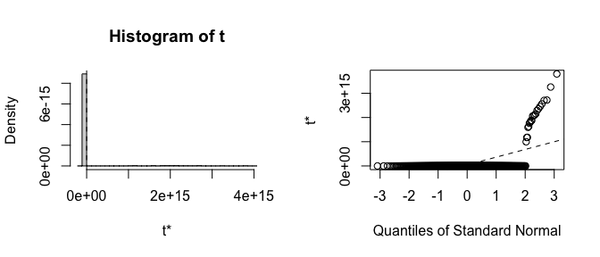
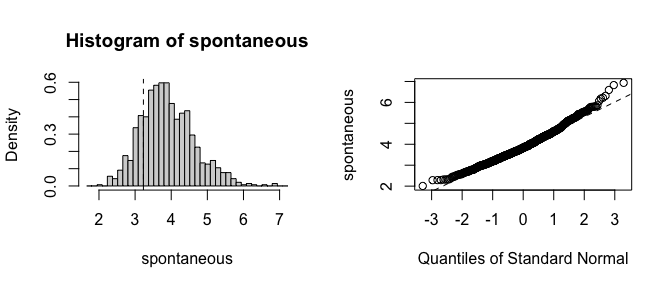
Already the bias and standard errors indicate problems with the traditional bootstrap. Let’s plot histograms of the estimates to see where the failure is:
plot(boot_est, index = 2)
plot(fwb_est, index = 2)
It is clear that the estimates from the traditional bootstrap are pathological, whereas the estimates from the FWB are more reasonable. The non-normality of the FWB distributions also suggests that the usual Wald-style confidence intervals may not be accurate, and a bias-corrected percentile interval should probably be computed instead.
fwb also contains utility functions for computing
weighted statistics to facilitate incorporation of bootstrapped weights
into estimates. These include w_mean(),
w_var(), w_sd(), w_quantile(),
and w_median() for computing weighted means, variances,
standard deviations, quantiles, and medians; w_cov() and
w_cor() for computing weighted covariance and correlation
matrices, and w_std(), w_scale(), and
w_center() for transforming variables by standardizing,
scaling, and centering using weighted statistics. Many of these serve as
drop-ins for base R functions, like weighted.mean() for
computing the weighted mean, but have the advantage that the weights do
not need to be manually supplied: when the functions are called from
within fwb() or vcovFWB(), the bootstrap
weights are automatically incorporated.
The FWB is uniformly more reliable than the traditional bootstrap when a weighted statistic can be computed (though this doesn’t mean the bootstrap is always valid). In most simple cases, both methods will yield the same results. In some pathological examples like those above, the FWB dramatically outperforms the traditional bootstrap. This will be true when running regression models with sparse categorical variables either in the outcome or among the predictors, for example, when estimating fixed effects or when a binary outcome is rare. However, it is important to know when a weighted statistic can be computed; for example, computing the weighted median is not always straightforward, making the traditional bootstrap potentially more useful for computing it. Still, though, the FWB deserves a place in an analyst’s toolbox.
boot, which provides the traditional bootstrap,
including an interface that accepts frequency weights to compute
weighted statistics, as was used abovebayesboot, which also provides functionality for the
Bayesian bootstrap but does so in a more explicitly Bayesian fashion and
with returned objects that are less consistent with those from
bootfwbTo cite fwb, please use citation("fwb"),
which generates a package citation.
Trichopoulos, D., Handanos, N., Danezis, J., Kalandidi, A. and Kalapothaki, V. (1976), Induced Abortion and Secondary Infertility. BJOG: An International Journal of Obstetrics & Gynaecology, 83, 645-650. https://doi.org/10.1111/j.1471-0528.1976.tb00904.x
Xu, L., Gotwalt, C., Hong, Y., King, C. B., & Meeker, W. Q. (2020). Applications of the Fractional-Random-Weight Bootstrap. The American Statistician, 74(4), 345–358. https://doi.org/10.1080/00031305.2020.1731599
These binaries (installable software) and packages are in development.
They may not be fully stable and should be used with caution. We make no claims about them.
Health stats visible at Monitor.