The hardware and bandwidth for this mirror is donated by dogado GmbH, the Webhosting and Full Service-Cloud Provider. Check out our Wordpress Tutorial.
If you wish to report a bug, or if you are interested in having us mirror your free-software or open-source project, please feel free to contact us at mirror[@]dogado.de.
![]()
The goal of flexCountReg is to provide functions that allow the analyst to estimate count regression models that can handle multiple analysis issues including excess zeros, overdispersion as a function of variables (i.e., generalized count models), random parameters, etc.
You can install the development version of flexCountReg like using:
# install.packages("devtools")
devtools::install_github("jwood-iastate/flexCountReg")The following functions are included in the flexCountReg
package, grouped by continuous and count distributions.
Distribution Functions
Continuous Distributions
Inverse Gamma Distribution
dinvgamma for the density functionpinvgamma for the cumulative density functionqinvgamma for the quantile functionrinvgamma for random number generationTriangle Distribution
dtri for the density functionptri for the cumulative density functionqtri for the quantile functionrtri for random number generationLognormal Distribution
mgf_lognormal for estimating the moment generating
functionCount Distributions
Generalized Waring Distribution
dgwar for the density functionpgwar for the cumulative density functionqgwar for the quantile functionrgwar for random number generationPoisson-Generalized-Exponential Distribution
dpge for the density functionppge for the cumulative density functionqpge for the quantile functionrpge for random number generationPoisson-Inverse-Gaussian Distribution (Types 1 and 2)
dpinvgaus for the density functionppinvgaus for the cumulative density functionqpinvgaus for the quantile functionrpinvgaus for random number generationPoisson-Inverse-Gamma Distribution
dpinvgamma for the density functionppinvgamma for the cumulative density functionqpinvgamma for the quantile functionrpinvgamma for random number generationPoisson-Lindley Distribution
dplind for the density functionpplind for the cumulative density functionqplind for the quantile functionrplind for random number generationPoisson-Lindley-Gamma (Negative Binomial-Lindley) Distribution
dplindGamma for the density functionpplindGamma for the cumulative density functionqplindGamma for the quantile functionrplindGamma for random number generationPoisson-Lindley-Lognormal Distribution
dplindLnorm for the density functionpplindLnorm for the cumulative density functionqplindLnorm for the quantile functionrplindLnorm for random number generationPoisson-Lognormal Distribution
dpLnorm for the density functionppLnorm for the cumulative density functionqtpLnorm for the quantile functionrpLnorm for random number generationPoisson-Weibull Distribution
dpoisweibull for the density functionppoisweibull for the cumulative density functionqpoisweibull for the quantile functionrpoisweibull for random number generationSichel Distribution
dsichel for the density functionpsichel for the cumulative density functionqsichel for the quantile functionrsichel for random number generationConway-Maxwell-Poisson Distribution
dcom for the density functionpcom for the cumulative density functionqcom for the quantile functionrcom for random number generationModel Estimation Functions
countreg is a general function for estimating the
non-panel, non-random parameters count regression modelscountreg.rp estimates the random parameters count
models.poislind.re estimates the random effects
Poisson-Lindley modelrenb estimates the random effects negative binomial
regression model.Model Evaluation, Comparison, and Convenience Functions
cureplot generates a CURE plot for the specified model,
based on the cureplots
package.mae computes the Mean Absolute Error (MAE).myAIC computes the Akaike Information Criterion (AIC)
value.myBIC computes the Bayesian Information Criterion (BIC)
value.regCompTable creates a publication-ready table
comparing multiple models. This can include the regression estimate
results, AIC, BIC, and Pseudo R-Square values.regCompTest compares any given model with a base model.
This can be used to perform a likelihood ratio test between models.rmse computes the Root Mean Squared Error (RMSE).predict allows the predict function to be used for
out-of-sample predictions for any of the flexCountReg models.summary allows the use of the summary function to get a
model summary from a flexCountReg regression object.Data A dataset, washington_roads, is
included. It is based on a sample of Washington primary 2-lane roads
from the years 2016-2018. Data for the roads, traffic volumes (AADT) and
associated crashes were obtained from the Highway Safety
Information System (HSIS).
As noted in the list of functions, the probability distributions below are included in the flexCountReg package. Details of the distributions are provided in the documentation (help files).
Continuous Distributions
Count Distributions Distributions that Handle Equidispersion
Distributions that handle Underdispersion
Distributions that Handle Overdispersion
Distributions that Handle Excess Zeros
The following is an example of using flexCountReg to estimate a negative binomial (NB-2) regression model with the overdispersion parameter as a function of predictor variables:
library(gt) # used to format summary tables here
library(flexCountReg)
library(knitr)

data("washington_roads")
washington_roads$AADT10kplus <- ifelse(washington_roads$AADT > 10000, 1, 0)
gen.nb2 <- countreg(Total_crashes ~ lnaadt + lnlength + speed50 + AADT10kplus,
               data = washington_roads, family = "NB2",
dis_param_formula_1 = ~ speed50, method='BFGS')kable(summary(gen.nb2), caption = "NB-2 Model Summary")
#> Call:
#> Total_crashes ~ lnaadt + lnlength + speed50 + AADT10kplus
#>
#> Method: countreg
#> Iterations: 44
#> Convergence: successful convergence
#> Log-likelihood: -1064.876
#>
#> Parameter Estimates:
#> (Using bootstrapped standard errors)
#> # A tibble: 7 × 7
#> parameter coeff `Std. Err.` `t-stat` `p-value` `lower CI` `upper CI`
#> <chr> <dbl> <dbl> <dbl> <dbl> <dbl> <dbl>
#> 1 (Intercept) -7.40 0.043 -172. 0 -7.49 -7.32
#> 2 lnaadt 0.912 0.005 182. 0 0.902 0.921
#> 3 lnlength 0.843 0.037 22.9 0 0.771 0.915
#> 4 speed50 -0.47 0.102 -4.62 0 -0.669 -0.27
#> 5 AADT10kplus 0.77 0.089 8.61 0 0.594 0.945
#> 6 ln(alpha):(Interc… -1.62 0.291 -5.57 0 -2.19 -1.05
#> 7 ln(alpha):speed50 1.31 0.458 2.85 0.004 0.409 2.20| parameter | coeff | Std. Err. | t-stat | p-value | lower CI | upper CI |
|---|---|---|---|---|---|---|
| (Intercept) | -7.401 | 0.043 | -171.562 | 0.000 | -7.486 | -7.317 |
| lnaadt | 0.912 | 0.005 | 182.453 | 0.000 | 0.902 | 0.921 |
| lnlength | 0.843 | 0.037 | 22.878 | 0.000 | 0.771 | 0.915 |
| speed50 | -0.470 | 0.102 | -4.619 | 0.000 | -0.669 | -0.270 |
| AADT10kplus | 0.770 | 0.089 | 8.607 | 0.000 | 0.594 | 0.945 |
| ln(alpha):(Intercept) | -1.619 | 0.291 | -5.568 | 0.000 | -2.189 | -1.049 |
| ln(alpha):speed50 | 1.306 | 0.458 | 2.854 | 0.004 | 0.409 | 2.203 |
NB-2 Model Summary
teststats <- regCompTest(gen.nb2)
kable(teststats$statistics)| Statistic | Model | BaseModel |
|---|---|---|
| AIC | 2143.7522 | 3049.659 |
| BIC | 2180.9494 | 3054.973 |
| LR Test Statistic | 917.9070 | NA |
| LR degrees of freedom | 6.0000 | NA |
| LR p-value | 0.0000 | NA |
| McFadden’s Pseudo R^2 | 0.3012 | NA |
Checking the CURE plot:
cureplot(gen.nb2, indvar  ="lnaadt")
#> Covariate: indvar_values
#> CURE data frame was provided. Its first column, lnaadt, will be used.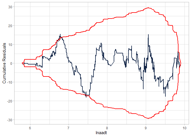
Modifying the model to fit better:
gen.nb2 <- countreg(Total_crashes ~ lnaadt  + lnlength + speed50 +
                                ShouldWidth04 + AADT10kplus +
                                I(AADT10kplus/lnaadt),
                                data = washington_roads, family = "NB2",
                                dis_param_formula_1 = ~ lnlength,  method='BFGS')

kable(summary(gen.nb2), caption = "Modified NB-2 Model Summary")
#> Call:
#>  Total_crashes ~ lnaadt + lnlength + speed50 + ShouldWidth04 +      AADT10kplus + I(AADT10kplus/lnaadt)
#>
#>  Method:  countreg
#> Iterations:  56
#> Convergence:  successful convergence
#> Log-likelihood:  -1061.914
#>
#> Parameter Estimates:
#> (Using bootstrapped standard errors)
#> # A tibble: 9 × 7
#>   parameter           coeff `Std. Err.` `t-stat` `p-value` `lower CI` `upper CI`
#>   <chr>               <dbl>       <dbl>    <dbl>     <dbl>      <dbl>      <dbl>
#> 1 (Intercept)        -7.68        0.043  -180.       0         -7.76      -7.59
#> 2 lnaadt              0.93        0.005   188.       0          0.92       0.939
#> 3 lnlength            0.853       0.038    22.6      0          0.779      0.927
#> 4 speed50            -0.4         0.091    -4.38     0         -0.579     -0.221
#> 5 ShouldWidth04       0.261       0.06      4.36     0          0.143      0.378
#> 6 AADT10kplus         5.96        0.092    64.6      0          5.78       6.14
#> 7 I(AADT10kplus/ln… -50.1         0.938   -53.5      0        -52.0      -48.3
#> 8 ln(alpha):(Inter…  -1.91        0.324    -5.91     0         -2.55      -1.28
#> 9 ln(alpha):lnleng… -0.43 0.244 -1.76 0.078 -0.908 0.048| parameter | coeff | Std. Err. | t-stat | p-value | lower CI | upper CI |
|---|---|---|---|---|---|---|
| (Intercept) | -7.676 | 0.043 | -179.752 | 0.000 | -7.759 | -7.592 |
| lnaadt | 0.930 | 0.005 | 187.633 | 0.000 | 0.920 | 0.939 |
| lnlength | 0.853 | 0.038 | 22.585 | 0.000 | 0.779 | 0.927 |
| speed50 | -0.400 | 0.091 | -4.382 | 0.000 | -0.579 | -0.221 |
| ShouldWidth04 | 0.261 | 0.060 | 4.355 | 0.000 | 0.143 | 0.378 |
| AADT10kplus | 5.961 | 0.092 | 64.628 | 0.000 | 5.780 | 6.142 |
| I(AADT10kplus/lnaadt) | -50.133 | 0.938 | -53.454 | 0.000 | -51.971 | -48.295 |
| ln(alpha):(Intercept) | -1.913 | 0.324 | -5.910 | 0.000 | -2.547 | -1.278 |
| ln(alpha):lnlength | -0.430 | 0.244 | -1.764 | 0.078 | -0.908 | 0.048 |
Modified NB-2 Model Summary
teststats <- regCompTest(gen.nb2)
kable(teststats$statistics)| Statistic | Model | BaseModel |
|---|---|---|
| AIC | 2141.8278 | 3049.659 |
| BIC | 2189.6528 | 3054.973 |
| LR Test Statistic | 923.8314 | NA |
| LR degrees of freedom | 8.0000 | NA |
| LR p-value | 0.0000 | NA |
| McFadden’s Pseudo R^2 | 0.3031 | NA |
cureplot(gen.nb2, indvar  ="lnaadt")
#> Covariate: indvar_values
#> CURE data frame was provided. Its first column, lnaadt, will be used.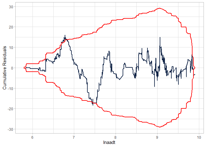
Estimating another model (NB-P) - without the interaction:
gen.nbp <- countreg(Total_crashes ~ lnaadt  + lnlength + speed50 +
                                ShouldWidth04 + AADT10kplus,
                                data = washington_roads, family = "NBp",
                                dis_param_formula_1 = ~ lnlength,  method='BFGS')
kable(summary(gen.nbp), caption = "NB-P Model Summary")
#> Call:
#>  Total_crashes ~ lnaadt + lnlength + speed50 + ShouldWidth04 +      AADT10kplus
#>
#>  Method:  countreg
#> Iterations:  53
#> Convergence:  successful convergence
#> Log-likelihood:  -1062.195
#>
#> Parameter Estimates:
#> (Using bootstrapped standard errors)
#> # A tibble: 9 × 7
#>   parameter           coeff `Std. Err.` `t-stat` `p-value` `lower CI` `upper CI`
#>   <chr>               <dbl>       <dbl>    <dbl>     <dbl>      <dbl>      <dbl>
#> 1 (Intercept)        -7.76        0.043 -181.        0         -7.85      -7.68
#> 2 lnaadt              0.938       0.005  189.        0          0.928      0.948
#> 3 lnlength            0.836       0.037   22.3       0          0.763      0.91
#> 4 speed50            -0.384       0.093   -4.13      0         -0.567     -0.202
#> 5 ShouldWidth04       0.258       0.059    4.34      0          0.141      0.374
#> 6 AADT10kplus         0.689       0.088    7.87      0          0.518      0.861
#> 7 ln(alpha):(Interc… -1.50        0.294   -5.09      0         -2.07      -0.92
#> 8 ln(alpha):lnlength -0.167       0.245   -0.682     0.495     -0.648      0.314
#> 9 ln(p) 0.525 0.173 3.03 0.002 0.186 0.864| parameter | coeff | Std. Err. | t-stat | p-value | lower CI | upper CI |
|---|---|---|---|---|---|---|
| (Intercept) | -7.764 | 0.043 | -181.211 | 0.000 | -7.848 | -7.680 |
| lnaadt | 0.938 | 0.005 | 189.459 | 0.000 | 0.928 | 0.948 |
| lnlength | 0.836 | 0.037 | 22.314 | 0.000 | 0.763 | 0.910 |
| speed50 | -0.384 | 0.093 | -4.130 | 0.000 | -0.567 | -0.202 |
| ShouldWidth04 | 0.258 | 0.059 | 4.335 | 0.000 | 0.141 | 0.374 |
| AADT10kplus | 0.689 | 0.088 | 7.867 | 0.000 | 0.518 | 0.861 |
| ln(alpha):(Intercept) | -1.496 | 0.294 | -5.094 | 0.000 | -2.072 | -0.920 |
| ln(alpha):lnlength | -0.167 | 0.245 | -0.682 | 0.495 | -0.648 | 0.314 |
| ln(p) | 0.525 | 0.173 | 3.033 | 0.002 | 0.186 | 0.864 |
NB-P Model Summary
teststats <- regCompTest(gen.nbp)
kable(teststats$statistics)| Statistic | Model | BaseModel |
|---|---|---|
| AIC | 2142.3895 | 3049.659 |
| BIC | 2190.2144 | 3054.973 |
| LR Test Statistic | 923.2697 | NA |
| LR degrees of freedom | 8.0000 | NA |
| LR p-value | 0.0000 | NA |
| McFadden’s Pseudo R^2 | 0.3029 | NA |
Checking the CURE plot (notice that the CURE plot is MUCH better in this case than the NB-2 without the interaction and still better than the modified NB-2):
cureplot(gen.nbp, indvar  ="lnaadt")
#> Covariate: indvar_values
#> CURE data frame was provided. Its first column, lnaadt, will be used.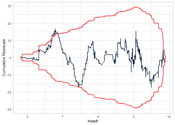
Creating a table to compare the models:
regCompTable(list("Generalized NB-2"=gen.nb2, "Generalized NB-P"=gen.nbp), tableType="tibble") |>
kable()| Parameter | Generalized NB-2 | Generalized NB-P |
|---|---|---|
| (Intercept) | -7.676 (0.043)*** | -7.764 (0.043)*** |
| lnaadt | 0.93 (0.005)*** | 0.938 (0.005)*** |
| lnlength | 0.853 (0.038)*** | 0.836 (0.037)*** |
| speed50 | -0.4 (0.091)*** | -0.384 (0.093)*** |
| ShouldWidth04 | 0.261 (0.06)*** | 0.258 (0.059)*** |
| AADT10kplus | 5.961 (0.092)*** | 0.689 (0.088)*** |
| I(AADT10kplus/lnaadt) | -50.133 (0.938)*** | — |
| ln(alpha):(Intercept) | -1.913 (0.324)*** | -1.496 (0.294)*** |
| ln(alpha):lnlength | -0.43 (0.244) | -0.167 (0.245) |
| ln(p) | — | 0.525 (0.173)** |
| N Obs. | 1501 | 1501 |
| LL | -1061.914 | -1062.195 |
| AIC | 2141.828 | 2142.389 |
| BIC | 2189.653 | 2190.214 |
| Pseudo-R-Sq. | 0.303 | 0.303 |
Note that the metrics for comparison are similar. While the models both have the same number of parameters, the NB-P was able to get better performance without requiring the interaction terms (which leads to strange relationships between the exposure metric and the outcome).
These binaries (installable software) and packages are in development.
They may not be fully stable and should be used with caution. We make no claims about them.
Health stats visible at Monitor.