The hardware and bandwidth for this mirror is donated by dogado GmbH, the Webhosting and Full Service-Cloud Provider. Check out our Wordpress Tutorial.
If you wish to report a bug, or if you are interested in having us mirror your free-software or open-source project, please feel free to contact us at mirror[@]dogado.de.
EQ-5D is a popular health related quality of life instrument used in the clinical and economic evaluation of health care. Developed by the EuroQol group, the instrument consists of two components: health state description and evaluation.
For the description component a subject self-rates their health in terms of five dimensions; mobility, self-care, usual activities, pain/discomfort, and anxiety/depression using either a three-level (EQ-5D-3L and EQ-5D-Y-3L) or a five-level (EQ-5D-5L) scale.
The evaluation component requires a patient to record their overall health status using a visual analogue scale (EQ-VAS).
Following assessment the scores from the descriptive component can be reported as a five digit number ranging from 11111 (full health) to 33333/55555 (worst health). A number of methods exist for analysing these five digit profiles. However, frequently they are converted to a single utility index using country specific value sets, which can be used in the clinical and economic evaluation of health care as well as in population health surveys.
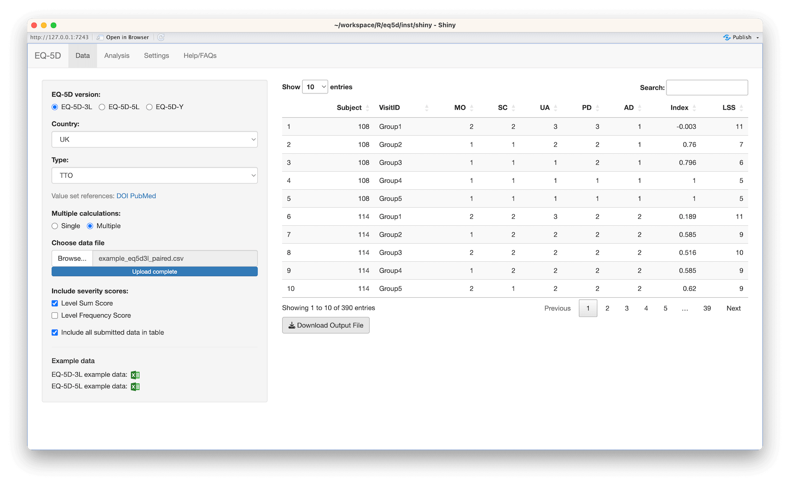
The eq5d package provides methods for the cross-sectional and longitudinal analysis of EQ-5D profiles and also the calculation of utility index scores from a subject’s dimension scores. Additionally, a Shiny app is included to enable the calculation, visualisation and automated statistical analysis of multiple EQ-5D index values via a web browser using EQ-5D dimension scores stored in CSV or Excel files.
Value sets for EQ-5D-3L are available for many countries and have been produced using the time trade-off (TTO) valuation technique or the visual analogue scale (VAS) valuation technique. Some countries have TTO and VAS value sets for EQ-5D-3L. Additionally, EQ-5D-3L “reverse crosswalk” value sets based on the van Hout et al (2021) models as well as those published on the EuroQol website that enable EQ-5D-3L data to be mapped to EQ-5D-5L value sets are included.
For EQ-5D-5L, a standardised valuation study protocol (EQ-VT) was developed by the EuroQol group based on the composite time trade-off (cTTO) valuation technique supplemented by a discrete choice experiment (DCE). The EuroQol group recommends users to use a standard value set where available.
The EQ-5D-5L “crosswalk” value sets published by van Hout et al (2012) as well as that for Russia are also included. The crosswalk value sets enable index values to be calculated for EQ-5D-5L data where no value set is available by mapping between the EQ-5D-5L and EQ-5D-3L descriptive systems.
The recently published age and sex conditional based mapping data by the NICE Decision Support Unit are also now part of the package. These enable age-sex based EQ-5D-3L to EQ-5D-5L and EQ-5D-5L to EQ-5D-3L mappings from dimensions and exact or approximate utility index scores.
Additional information on EQ-5D can be found on the EuroQol website as well as in Szende et al (2007) and Szende et al (2014). Advice on choosing a value set can also be found on the EuroQol website.
You can install the released version of eq5d from CRAN with:
install.packages("eq5d")And the development version from GitHub with:
# install.packages("devtools")
devtools::install_github("fragla/eq5d")library(eq5d)
#> Loading required package: lifecycle
#> Loading required package: rlang
#single calculation
#named vector MO, SC, UA, PD and AD represent mobility, self-care, usual activites, pain/discomfort and anxiety/depression, respectfully.
scores <- c(MO=1,SC=2,UA=3,PD=2,AD=1)
#EQ-5D-3L using the UK TTO value set
eq5d(scores=scores, country="UK", version="3L", type="TTO")
#> [1] 0.329
#Using five digit format
eq5d(scores=12321, country="UK", version="3L", type="TTO")
#> [1] 0.329
#EQ-5D-Y-3L using the Slovenian value set
eq5d(scores=13321, country="Slovenia", version="Y3L")
#> [1] 0.295
#EQ-5D-5L crosswalk
eq5d(scores=55555, country="Spain", version="5L", type="CW")
#> [1] -0.654
#EQ-5D-3L reverse crosswalk
eq5d(scores=33333, country="Germany", version="3L", type="RCW")
#> [1] -0.495
#EQ-5D-5L to EQ-5D-3L NICE DSU mapping
#Using dimensions
eq5d(c(MO=1,SC=2,UA=3,PD=4,AD=5), version="5L", type="DSU", country="UK", age=23, sex="male")
#> [1] 0.083
#Using exact utility score
eq5d(0.922, country="UK", version="5L", type="DSU", age=18, sex="male")
#> [1] 0.893
#Using approximate utility score
eq5d(0.435, country="UK", version="5L", type="DSU", age=30, sex="female", bwidth=0.0001)
#> [1] 0.302
#multiple calculations using the Canadian VT value set
#data.frame with individual dimensions
scores.df <- data.frame(
MO=c(1,2,3,4,5), SC=c(1,5,4,3,2), UA=c(1,5,2,3,1), PD=c(1,3,4,3,4), AD=c(1,2,1,2,1)
)
eq5d(scores.df, country="Canada", version="5L", type="VT")
#> [1] 0.949 0.362 0.390 0.524 0.431
#data.frame using five digit format
scores.df2 <- data.frame(state=c(11111, 25532, 34241, 43332, 52141))
eq5d(scores.df2, country="Canada", version="5L", type="VT", five.digit="state")
#> [1] 0.949 0.362 0.390 0.524 0.431
#or using a vector
eq5d(scores.df2$state, country="Canada", version="5L", type="VT")
#> [1] 0.949 0.362 0.390 0.524 0.431The available value sets can be viewed using the valuesets function. The results can be filtered by EQ-5D version, value set type or by country.
# Return TTO value sets with PubMed IDs and DOIs (top 6 returned for brevity).
head(valuesets(type="TTO", references=c("PubMed","DOI")))
#>    Version Type   Country   PubMed                              DOI
#> 1 EQ-5D-3L  TTO Argentina 19900257 10.1111/j.1524-4733.2008.00468.x
#> 2 EQ-5D-3L  TTO Australia 21914515       10.1016/j.jval.2011.04.009
#> 3 EQ-5D-3L  TTO   Bermuda 38982011       10.1007/s10198-024-01701-2
#> 4 EQ-5D-3L  TTO    Brazil 29702778       10.1016/j.vhri.2013.01.009
#> 5 EQ-5D-3L  TTO    Canada 22328929     10.1371/journal.pone.0031115
#> 6 EQ-5D-3L  TTO     Chile 22152184      10.1016/j.jval.2011.09.002.

# Return VAS value sets with ISBN and external URL (top 6 returned for brevity).
head(valuesets(type="VAS", references=c("ISBN","ExternalURL")))
#>    Version Type Country          ISBN
#> 1 EQ-5D-3L  VAS Belgium 1-4020-5511-0
#> 2 EQ-5D-3L  VAS Denmark 1-4020-5511-0
#> 3 EQ-5D-3L  VAS  Europe 1-4020-5511-0
#> 4 EQ-5D-3L  VAS Finland 1-4020-5511-0
#> 5 EQ-5D-3L  VAS Germany 1-4020-5511-0
#> 6 EQ-5D-3L  VAS    Iran          <NA>
#>                                                              ExternalURL
#> 1 https://eq-5dpublications.euroqol.org/download?id=0_54011&fileId=54420
#> 2 https://eq-5dpublications.euroqol.org/download?id=0_54011&fileId=54420
#> 3 https://eq-5dpublications.euroqol.org/download?id=0_54011&fileId=54420
#> 4 https://eq-5dpublications.euroqol.org/download?id=0_54011&fileId=54420
#> 5 https://eq-5dpublications.euroqol.org/download?id=0_54011&fileId=54420
#> 6                                                                   <NA>

# Return EQ-5D-5L value sets (top 6 returned for brevity).
head(valuesets(version="5L"))
#>    Version Type Country   PubMed                        DOI ISBN ExternalURL
#> 1 EQ-5D-5L   CW Bermuda 38982011 10.1007/s10198-024-01701-2 <NA>        <NA>
#> 2 EQ-5D-5L   CW Denmark 22867780 10.1016/j.jval.2012.02.008 <NA>        <NA>
#> 3 EQ-5D-5L   CW  France 22867780 10.1016/j.jval.2012.02.008 <NA>        <NA>
#> 4 EQ-5D-5L   CW Germany 22867780 10.1016/j.jval.2012.02.008 <NA>        <NA>
#> 5 EQ-5D-5L   CW   Japan 22867780 10.1016/j.jval.2012.02.008 <NA>        <NA>
#> 6 EQ-5D-5L   CW  Jordan 39225720 10.1007/s10198-024-01712-z <NA>        <NA>

# Return all French value sets.
valuesets(country="France")
#>    Version Type Country   PubMed                        DOI ISBN ExternalURL
#> 1 EQ-5D-3L  TTO  France 21935715  10.1007/s10198-011-0351-x <NA>        <NA>
#> 2 EQ-5D-5L   CW  France 22867780 10.1016/j.jval.2012.02.008 <NA>        <NA>
#> 3 EQ-5D-5L   VT  France 31912325 10.1007/s40273-019-00876-4 <NA>        <NA>
#> 4 EQ-5D-3L  RCW  France 34452708 10.1016/j.jval.2021.03.009 <NA>        <NA>
#>             Notes
#> 1            <NA>
#> 2            <NA>
#> 3            <NA>
#> 4 van Hout (2021)

# Return all EQ-5D-5L to EQ-5D-3L DSU value sets without references.
valuesets(type="DSU", version="5L", references=NULL)
#>    Version Type     Country
#> 1 EQ-5D-5L  DSU       China
#> 2 EQ-5D-5L  DSU     Germany
#> 3 EQ-5D-5L  DSU       Japan
#> 4 EQ-5D-5L  DSU Netherlands
#> 5 EQ-5D-5L  DSU  SouthKorea
#> 6 EQ-5D-5L  DSU       Spain
#> 7 EQ-5D-5L DSU UKA number of methods have been published that enable the analysis of EQ-5D profiles, most recently in the open access book Methods for Analysing and Reporting EQ-5D Data by Devlin, Janssen and Parkin. The eq5d package includes R implentations of some of the methods from this book and from other sources that may be of use in analysing EQ-5D data.
The eq5dcf function calculates the frequency, percentage, cumulative frequency and cumulative percentage for each five digit profile in an EQ-5D dataset. Either a vector of five digit profiles or a data.frame of individual dimensions can be passed to this function in order to summarise data in this way.
library(readxl)

#load example data
data <- read_excel(system.file("extdata", "eq5d3l_example.xlsx", package="eq5d"))

#run eq5dcf function on a data.frame
res <- eq5dcf(data, "3L")

# Return data.frame of cumulative frequency stats (top 6 returned for brevity).
head(res)
#>   State Frequency Percentage CumulativeFreq CumulativePerc
#> 1 11121        36       18.0             36           18.0
#> 2 11111        24       12.0             60           30.0
#> 3 22222        21       10.5             81           40.5
#> 4 22221        18        9.0             99           49.5
#> 5 11221        12        6.0            111           55.5
#> 6 21221 11 5.5 122 61.0The eq5d package includes methods for summarising the severity of EQ-5D health state. The Level Sum Score (LSS) treats each dimension’s level as a number rather than a category. Each number is added up to produce a score between 5 and 15 for EQ-5D-3L and 5 and 25 for EQ-5D-5L.
lss(c(MO=1,SC=2,UA=3,PD=2,AD=1), version="3L")
#> [1] 9

lss(55555, version="5L")
#> [1] 25

lss(c(11111, 12345, 55555), version="5L")
#> [1]  5 15 25
The Level Frequency Score (LFS) is an alternative method of summarising profile data developed by Oppe and de Charro. Here the frequency of the levels for each health state are characterised. As described in Devlin, Janssen and Parkin’s book, the full health profile 11111 for EQ-5D-5L has 5, 1 s, no level 2, 3, 4 and 5s, so the LFS is 50000; the health profile 55555 is 00005; profiles such as 31524 and 53412 would be 11111.
lfs(c(MO=1,SC=2,UA=3,PD=2,AD=1), version="3L")
#> [1] "221"

lfs(55555, version="5L")
#> [1] "00005"

lfs(c(11111, 12345, 55555), version="5L")
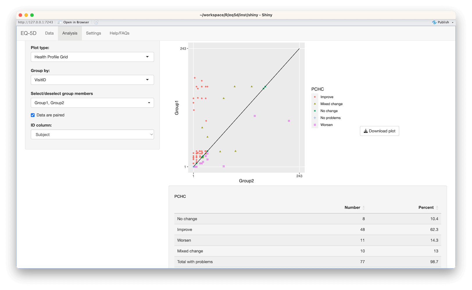
#> [1] "50000" "11111" "00005"The Paretian Classification of Health Change (PCHC) was developed by Devlin et al in 2010 and is used to compare changes in individuals over time. PCHC classifies the change in an individual’s health state as better (improvement in at least one dimension), worse (a deterioration in at least one dimension), mixed (improvements and deteriorations in dimensions) or there being no change in the health state. Those classified in the No change group with the 11111 health state can be separated into their own “No problems” group. PCHC can be calculated using the pchc function.
library(readxl)

#load example data
data <- read_excel(system.file("extdata", "eq5d3l_example.xlsx", package="eq5d"))

#use first 50 entries of each group as pre/post
pre <- data[data$Group=="Group1",][1:50,]
post <- data[data$Group=="Group2",][1:50,]

#run pchc function on data.frames

#Show no change, improve, worse, mixed without totals
res1 <- pchc(pre, post, version="3L", no.problems=FALSE, totals=FALSE)
res1
#>              Number Percent
#> No change         5      10
#> Improve          32      64
#> Worsen           10      20
#> Mixed change      3       6

#Show totals, but not those with no problems
res2 <- pchc(pre, post, version="3L", no.problems=FALSE, totals=TRUE)
res2
#>              Number Percent
#> No change         5      10
#> Improve          32      64
#> Worsen           10      20
#> Mixed change      3       6
#> Total            50     100

#Show totals and no problems for each dimension
res3 <- pchc(pre, post, version="3L", no.problems=TRUE, totals=TRUE, by.dimension=TRUE)
res3
#> $MO
#>                     Number Percent
#> No change               16    57.1
#> Improve                 11    39.3
#> Worsen                   1     3.6
#> Total with problems     28    56.0
#> No problems             22    44.0
#>
#> $SC
#>                     Number Percent
#> No change               10    37.0
#> Improve                 14    51.9
#> Worsen                   3    11.1
#> Total with problems     27    54.0
#> No problems             23    46.0
#>
#> $UA
#>                     Number Percent
#> No change               10      25
#> Improve                 26      65
#> Worsen                   4      10
#> Total with problems     40      80
#> No problems             10      20
#>
#> $PD
#>                     Number Percent
#> No change               27    57.4
#> Improve                 19    40.4
#> Worsen                   1     2.1
#> Total with problems     47    94.0
#> No problems              3     6.0
#>
#> $AD
#>                     Number Percent
#> No change                7    30.4
#> Improve                  9    39.1
#> Worsen                   7    30.4
#> Total with problems     23    46.0
#> No problems             27    54.0

#Don't summarise. Return all classifications
res4 <- pchc(pre, post, version="3L", no.problems=TRUE, totals=FALSE, summary=FALSE)
head(res4)
#> [1] "Improve"      "Improve"      "Improve"      "Improve"      "Improve"
#> [6] "Mixed change"The Probability of Superiority (PS) is a non-parametric measure of effect size introduced by Buchholz et al in 2015 and enables the assessment of paired samples of EQ-5D profile data in the context of assessing changes in health in terms of improvement or deterioration. For each EQ-5D dimension the number of subjects that have improved over time is divided by the total number of matched pairs. Ties (those with no changes) were accounted for through the addition of half the number of ties to the numerator. The score is less than 0.5 if more patients deteriorate than improve, 0.5 if the same number of patients improve and deteriorate or do not change and greater than 0.5 if more patients improve than deteriorate.
library(readxl)

#load example data
data <- read_excel(system.file("extdata", "eq5d3l_example.xlsx", package="eq5d"))

#use first 50 entries of each group as pre/post
pre <- data[data$Group=="Group1",][1:50,]
post <- data[data$Group=="Group2",][1:50,]

res <- ps(pre, post, version="3L")
res
#> $MO
#> [1] 0.6
#>
#> $SC
#> [1] 0.61
#>
#> $UA
#> [1] 0.72
#>
#> $PD
#> [1] 0.68
#>
#> $AD
#> [1] 0.52The Health Profile Grid (HPG) was also introduced by Devlin et al in 2010. The HPG provides a visual way to observe changes in individuals between two time points. The HPG requires profiles for each time point to be ordered from best to worst. The hpg function uses a specified value set for this with profiles being assigned a ranking between 1 and 243 for EQ-5D-3L and 1 and 3125 for EQ-5D-5L based on severity (1 being the best and 243/3125 the worst). The rankings for the two time points for each individual are plotted with the location of each point showing whether there has been an improvement or deterioration. The further a point is above the 45° line, the great the improvement in an individuals health. Conversely, the further below the line a point is the more health has deteriorated. Those individuals on the line show “no change”.
library(readxl)

#load example data
data <- read_excel(system.file("extdata", "eq5d3l_example.xlsx", package="eq5d"))

#use first 50 entries of each group as pre/post
pre <- data[data$Group=="Group1",][1:50,]
post <- data[data$Group=="Group2",][1:50,]

#run hpg function on data.frames

#Show pre/post rankings and PCHC classification
res <- hpg(pre, post, country="UK", version="3L", type="TTO")
head(res)
#>   Pre Post         PCHC
#> 1  11    8      Improve
#> 2 161    8      Improve
#> 3  23    1      Improve
#> 4  20    1      Improve
#> 5  23    9      Improve
#> 6  33   97 Mixed change

#Plot data using ggplot2
library(ggplot2)

ggplot(res, aes(Post, Pre, color=PCHC)) +
  geom_point(aes(shape=PCHC)) +
  coord_cartesian(xlim=c(1,243), ylim=c(1,243)) +
  scale_x_continuous(breaks=c(1,243)) +
  scale_y_continuous(breaks=c(1,243)) +
  annotate("segment", x=1, y=1, xend=243, yend=243, colour="black") +
  theme(panel.border=element_blank(), panel.grid.minor=element_blank()) +
  xlab("Post-treatment") +
  ylab("Pre-treatment")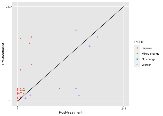
Shannon’s indices were first used to assess how evenly EQ-5D dimension scores or health states in a dataset are distributed by Janssen et al in 2007. Shannon’s H’ (diversity) index represents the absolute amount of informativity captured with Shannon’s J’ (evenness) index capturing the evenness of the distribution of data. Shannon’s J’ is calculated by dividing H’ by H’ max to give a value between 0 and 1. Lower values indicate more diversity and higher values indicate less.
library(readxl)

#load example data
data <- read_excel(system.file("extdata", "eq5d3l_example.xlsx", package="eq5d"))

#Shannon's H', H' max and J' for the whole dataset
shannon(data, version="3L", by.dimension=FALSE)
#> $H
#> [1] 4.17
#>
#> $H.max
#> [1] 7.92
#>
#> $J
#> [1] 0.53

#Shannon's H', H' max and J' for each dimension
res <- shannon(data, version="3L", by.dimension=TRUE)

#Convert to data.frame for ease of viewing
do.call(rbind, res)
#>    H    H.max J
#> MO 1    1.58  0.63
#> SC 0.97 1.58  0.61
#> UA 1.22 1.58  0.77
#> PD 1.13 1.58  0.71
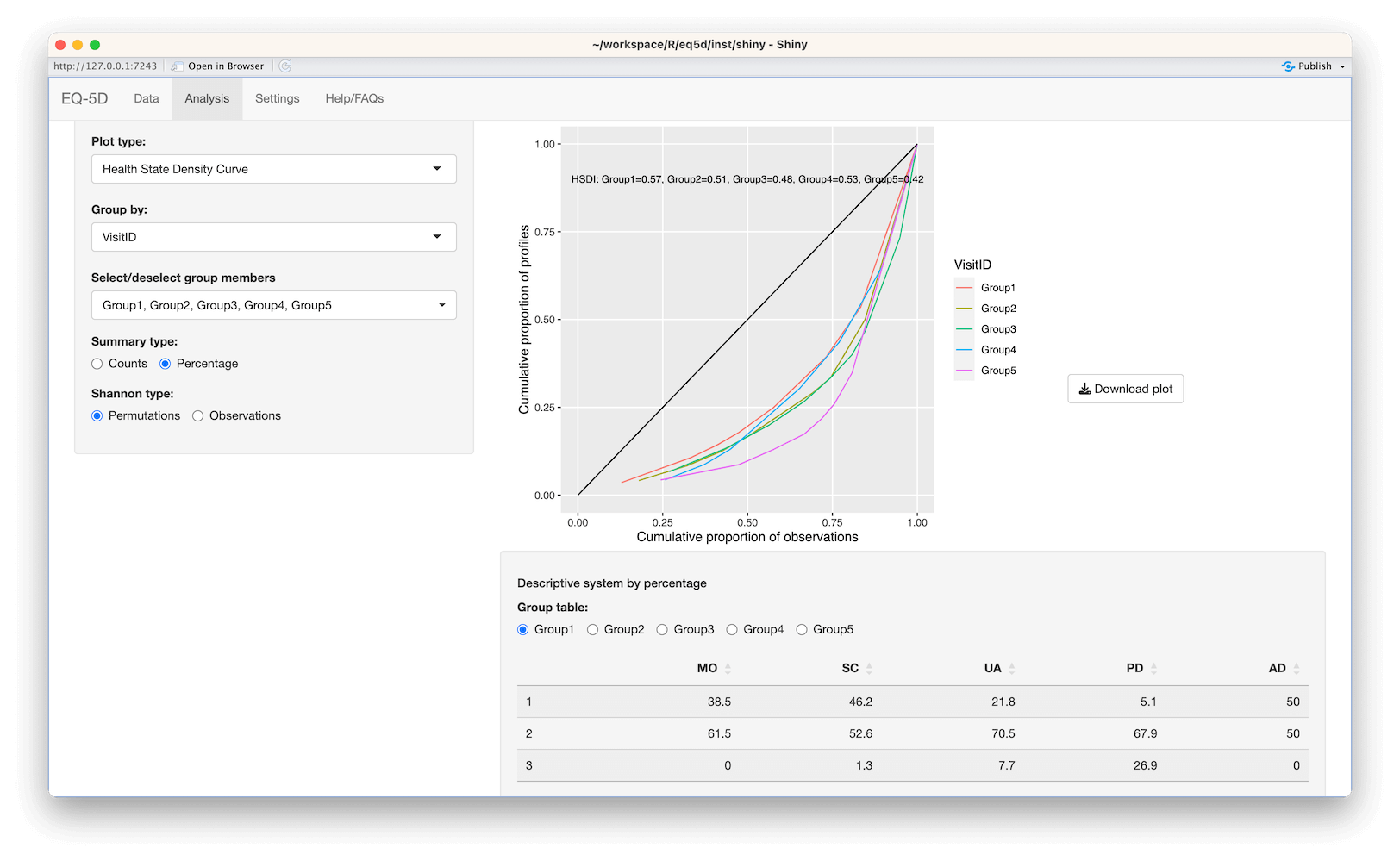
#> AD 1.09 1.58 0.69The Health State Density Curve (HSDC) was introduced by Zamora et al in 2018 and provides a graphical way to depict the distribution of EQ-5D profiles. The cumulative frequency of health profiles ranked from most to least frequent is plotted against the cumulative proportion of the distinct health profiles (red line) and can be compared a uniform distribution representing total equality (black line). The Health State Density Index (HSDI) is based on the area formed by the diagonal line representing total equality and the line of the HSDC. The HSDI has a value between 0 and 1 where a value of 0 represents total inequality and 1 total equality.
#load example data
data <- read_excel(system.file("extdata", "eq5d3l_example.xlsx", package="eq5d"))

#Calculate HSDI
hsdi <- hsdi(data, version="3L")

#Plot HSDC
cf <- eq5dcf(data, version="3L", proportions=T)
cf$CumulativeState <- 1:nrow(cf)/nrow(cf)

#Plot data using ggplot2
library(ggplot2)

ggplot(cf, aes(CumulativeProp, CumulativeState)) +
  geom_line(color="#FF9999") +
  annotate("segment", x=0, y=0, xend=1, yend=1, colour="black") +
  annotate("text", x=0.5, y=0.9, label=paste0("HSDI=", hsdi)) +
  theme(panel.border=element_blank(), panel.grid.minor=element_blank()) +
  coord_cartesian(xlim=c(0,1), ylim=c(0,1)) +
  xlab("Cumulative proportion of observations") +
  ylab("Cumulative proportion of profiles")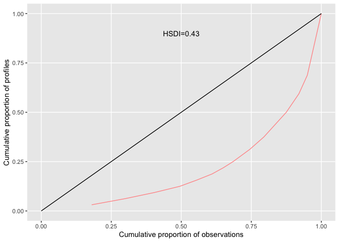
The eq5dds function is an R approximation of the Stata command written by Ramos-Goñi & Ramallo-Fariña. The function analyses and summarises the descriptive components of an EQ-5D dataset. The “by” argument enables a grouping variable to be specified when analysing the data subgroup.
set.seed(12345)
dat <- data.frame(
         matrix(
           sample(1:3, 5*12, replace=TRUE), 12, 5,
           dimnames=list(1:12, c("MO","SC","UA","PD","AD"))
         ),
         Sex=rep(c("Male", "Female"))
       )

eq5dds(dat, version="3L")
#>     MO   SC   UA   PD   AD
#> 1  8.3 33.3 33.3 41.7 16.7
#> 2 58.3 50.0 25.0 16.7 33.3
#> 3 33.3 16.7 41.7 41.7 50.0

eq5dds(dat, version="3L", counts=TRUE)
#>   MO SC UA PD AD
#> 1  1  4  4  5  2
#> 2  7  6  3  2  4
#> 3  4  2  5  5  6

eq5dds(dat, version="3L", by="Sex")
#> data[, by]: Female
#>     MO   SC   UA   PD   AD
#> 1  0.0 33.3 33.3 33.3  0.0
#> 2 66.7 50.0 33.3 16.7 16.7
#> 3 33.3 16.7 33.3 50.0 83.3
#> ------------------------------------------------------------
#> data[, by]: Male
#>     MO   SC   UA   PD   AD
#> 1 16.7 33.3 33.3 50.0 33.3
#> 2 50.0 50.0 16.7 16.7 50.0
#> 3 33.3 16.7 50.0 33.3 16.7
Helper functions are included, which may be useful in the processing of EQ-5D data. get_all_health_states returns a vector of all possible five digit health states for a specified EQ-5D version. get_dimensions_from_health_states splits a vector of five digit health states into a data.frame of their individual components and get_health_states_from_dimensions combines indiviual dimensions in a data.frame into five digit health states.
# Get all EQ-5D-3L five digit health states (top 6 returned for brevity).
head(get_all_health_states("3L"))
#> [1] "11111" "11112" "11113" "11121" "11122" "11123"

# Split five digit health states into their individual components.
get_dimensions_from_health_states(c("12345", "54321"), version="5L")
#>   MO SC UA PD AD
#> 1  1  2  3  4  5
#> 2  5  4  3  2  1
Example data is included with the package and can be accessed using the system.file function.
# View example files.
dir(path=system.file("extdata", package="eq5d"))
#> [1] "eq5d3l_example.csv"             "eq5d3l_example.xlsx"
#> [3] "eq5d3l_five_digit_example.csv"  "eq5d3l_five_digit_example.xlsx"
#> [5] "eq5d5l_example.csv"             "eq5d5l_example.xlsx"

# Read example EQ-5D-3L data.
library(readxl)
data <- read_excel(system.file("extdata", "eq5d3l_example.xlsx", package="eq5d"))

# Calculate index scores
scores <- eq5d(data, country="UK", version="3L", type="TTO")

# Top 6 scores
head(scores)
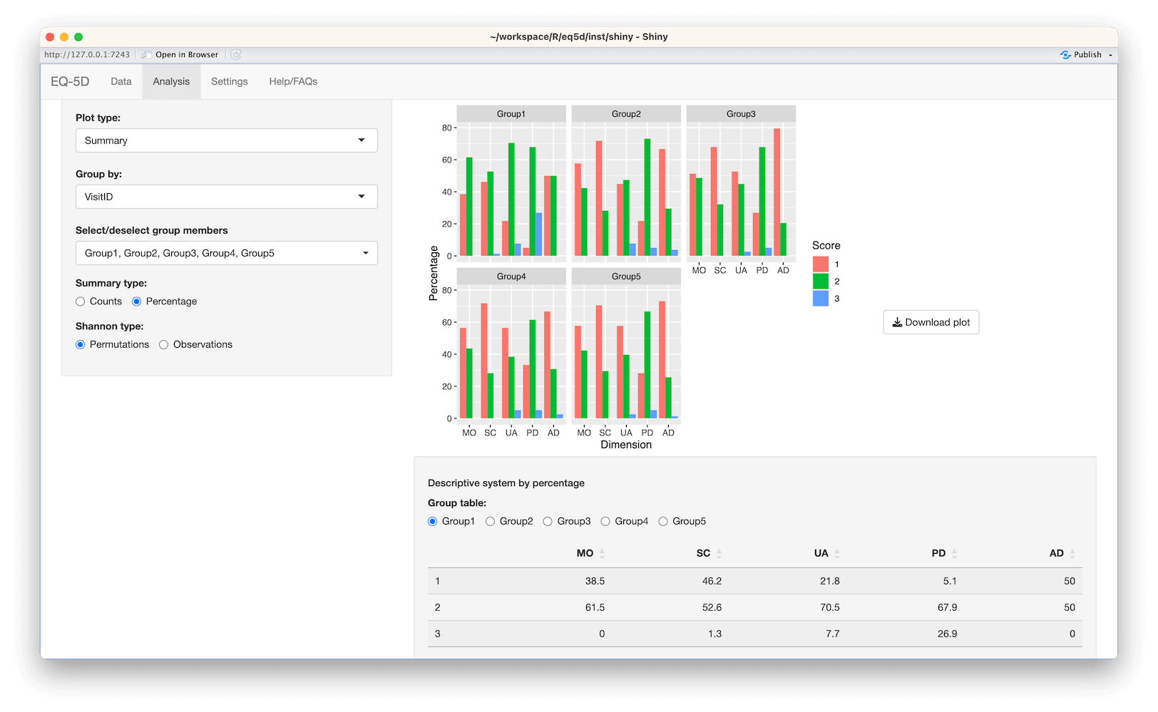
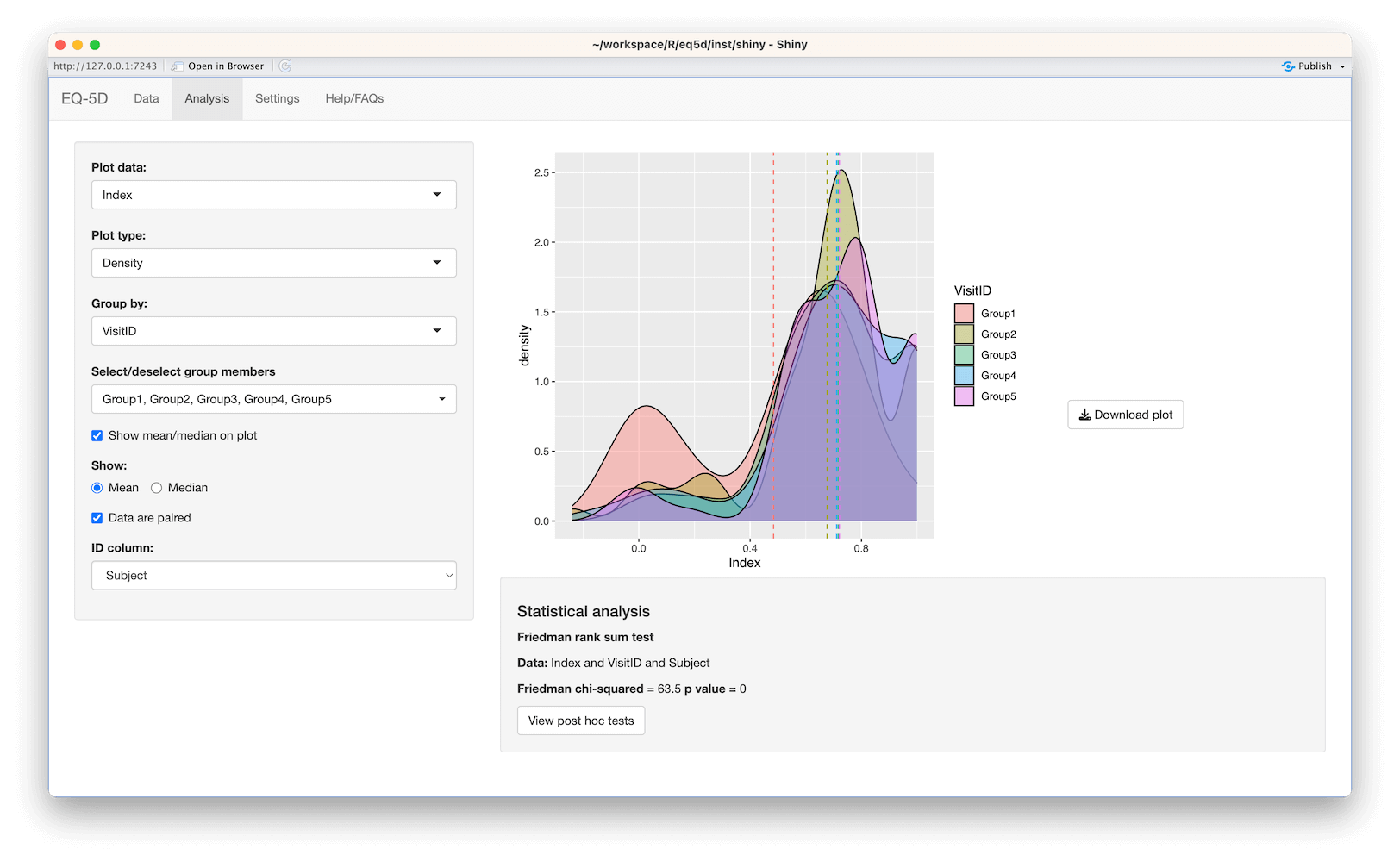
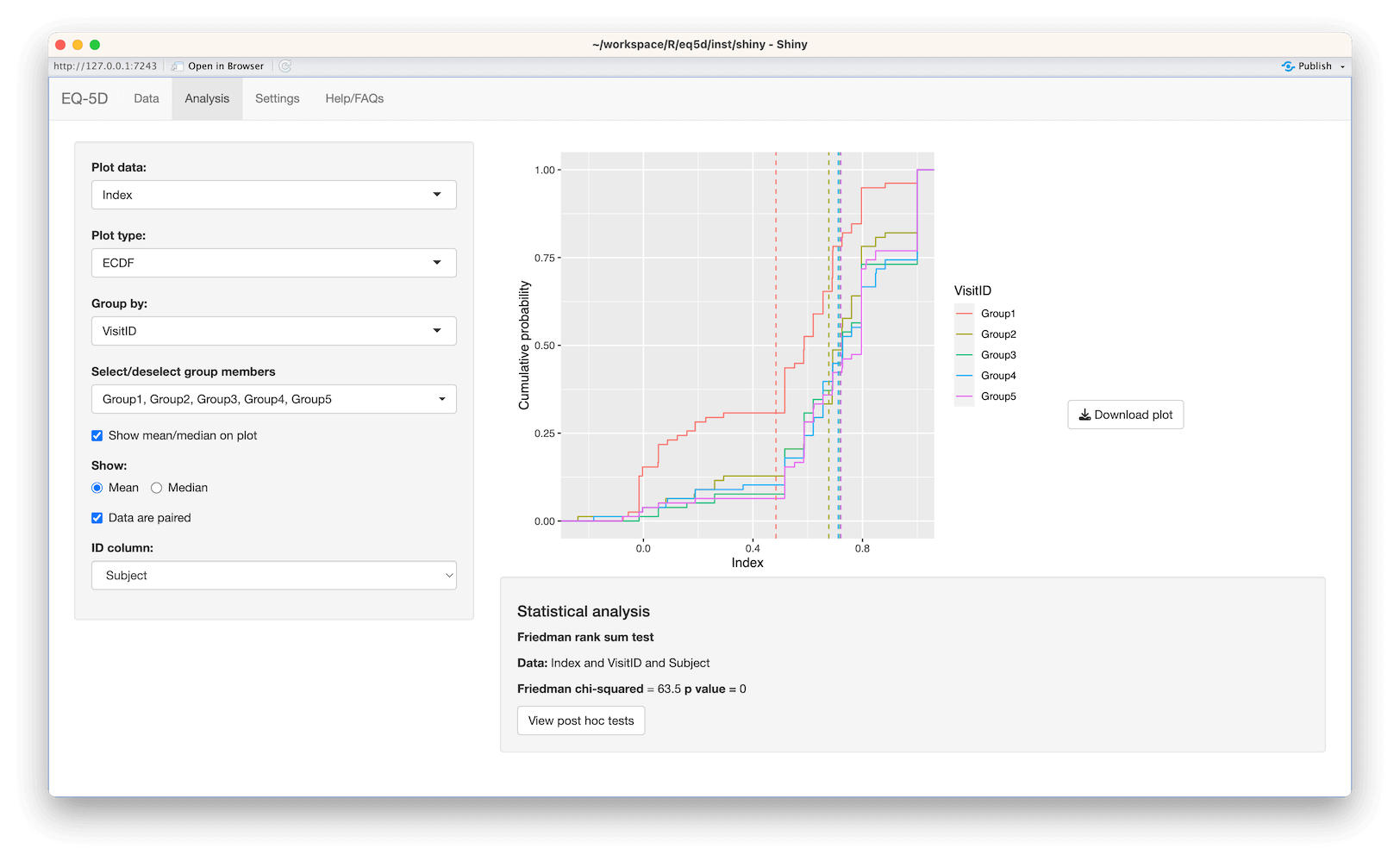
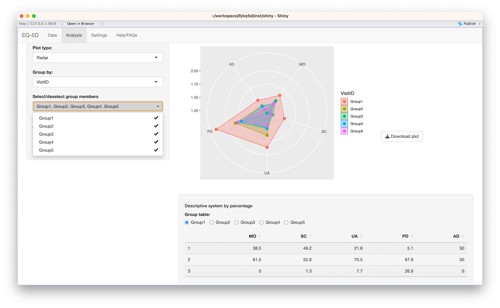
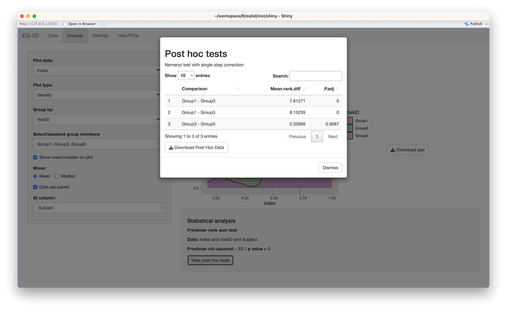
#> [1] 0.760 0.796 -0.003 0.796 0.656 1.000The calculation (and visualisation) of multiple EQ-5D indices can also be performed by upload of a CSV or Excel file using the packaged Shiny app. This requires the shiny, DT, FSA, ggplot2, ggiraph, ggiraphExtra, mime, PMCMRplus, readxl, shinycssloaders and shinyWidgets packages. Ideally the CSV/Excel headers should be the same as the names of the vector passed to the eq5d function i.e. MO, SC, UA, PD and AD or the column name “State” if using the five digit format. However, a modal dialog will prompt the user to select the appropriate columns if the defaults can not be found. Both files below will produce the same results.
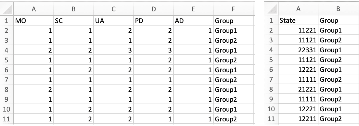
The app is launched using the shiny_eq5d function.
shiny_eq5d()Alternatively, it can be accessed without installing R/Shiny/eq5d by visiting shinyapps.io.
This project is licensed under the MIT License - see the LICENSE.md file for details.
These binaries (installable software) and packages are in development.
They may not be fully stable and should be used with caution. We make no claims about them.
Health stats visible at Monitor.