ecoregime

The hardware and bandwidth for this mirror is donated by dogado GmbH, the Webhosting and Full Service-Cloud Provider. Check out our Wordpress Tutorial.
If you wish to report a bug, or if you are interested in having us mirror your free-software or open-source project, please feel free to contact us at mirror[@]dogado.de.
ecoregime

ecoregime implements the EDR framework to characterize
and compare groups of ecological trajectories in multidimensional spaces
defined by ecosystem state variables. The EDR framework was introduced
in:
ecoregime can be used to assess ecological resilience
using ecological dynamic regimes as the system’s reference. This
approach was introduced in:
ecoregime includes functions to forecast ecological
trajectories from ecological dynamic regimes and assess the accuracy of
the predictions. This method was introduced in:
You can install ecoregime via CRAN:
install.packages("ecoregime")You can also install the development version of
ecoregime with:
# install.packages("devtools")
devtools::install_github("MSPinillos/ecoregime")
You can get an overview about its functionality and the workflow of the EDR framework in the package documentation and vignettes.
# Force the inclusion of the vignette in the installation
devtools::install_github("MSPinillos/ecoregime",
                         build_opts = c("--no-resave-data", "--no-manual"),
                         build_vignettes = TRUE)

# Load the package after the installation
library(ecoregime)

# Access the documentation and vignettes
?ecoregime
vignette("EDR_framework", package = "ecoregime")
vignette("Resilience", package = "ecoregime")
vignette("Predicting_trajectories", package = "ecoregime")Identify and plot representative trajectories in ecological dynamic regimes.
library(ecoregime)

# Calculate state dissimilarities from a matrix of state variables (e.g., species abundances)
variables <- data.frame(EDR_data$EDR3$abundance)
d <- vegan::vegdist(variables[, -c(1:3)])

# Identify the trajectory (or site) and states in d
trajectories <- variables$traj
states <- as.integer(variables$state)

# Compute RETRA-EDR
RT <- retra_edr(d = d, trajectories = trajectories, states = states,
                 minSegs = 5)

# Plot representative trajectories of the EDR
plot(x = RT, d = d, trajectories = trajectories, states = states, select_RT = "T4",
     traj.colors = "lightblue", RT.colors = "orange", sel.color = "darkgreen",
     link.lty = 1, asp = 1, xlab = "MDS D1", ylab = "MDS D2",
     main = "Representative trajectories - EDR")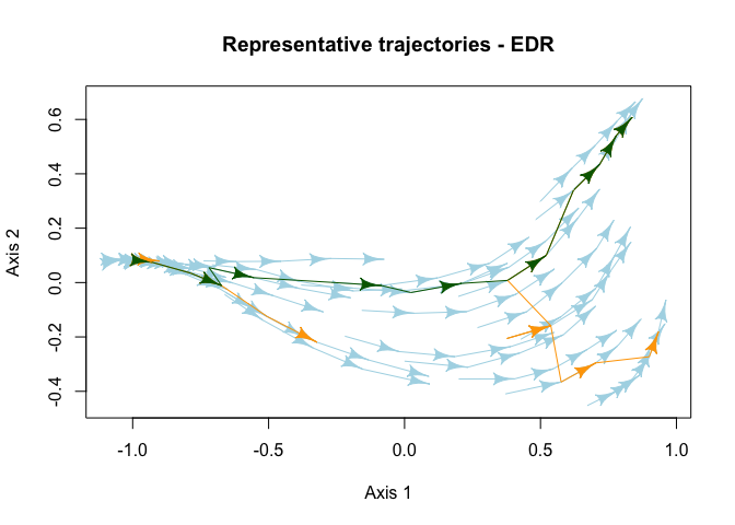
Characterize the internal structure of ecological dynamic regimes calculating the dispersion (dDis), beta diversity (dBD), and evenness (dEve) of the individual trajectories.
# Dynamic dispersion considering trajectory "1" as a reference
dDis(d = d, d.type = "dStates", trajectories = trajectories, states = states, reference = "1")
#> dDis (ref. 1)
#>     0.4083905

# Dynamic beta diversity
dBD(d = d, d.type = "dStates", trajectories = trajectories, states = states)
#>        dBD
#> 0.07946371

# Dynamic evenness
dEve(d = d, d.type = "dStates", trajectories = trajectories, states = states)
#>     dEve
#> 0.842375
Compare ecological dynamic regimes.
# Load species abundances and compile in a data frame
variables1 <- EDR_data$EDR1$abundance
variables2 <- EDR_data$EDR2$abundance
variables3 <- EDR_data$EDR3$abundance
all_variables <- data.frame(rbind(variables1, variables2, variables3))

# Calculate dissimilarities between every pair of states
d <- vegan::vegdist(all_variables[, -c(1:3)])

# Compute dissimilarities between EDRs:
dist_edr(d = d, d.type = "dStates",
         trajectories = all_variables$traj, states = all_variables$state,
         edr = all_variables$EDR, metric = "dDR", symmetrize = NULL)
#>           1         2         3
#> 1 0.0000000 0.5895458 0.6467200
#> 2 0.5700499 0.0000000 0.2768759
#> 3 0.6317846 0.5050273 0.0000000
Assess ecological resilience to pulse disturbances.
# Species abundances for disturbed communities
disturbed <- EDR_data$EDR3_disturbed$abundance[disturbed_states %in% c(0, 1, 14)]

# Species abundances for disturbed and reference communities
variables$disturbed_states <- 0
disturbed_ref <- rbind(variables, disturbed)

# Calculate dissimilarities between every pair of states
d <- vegan::vegdist(disturbed_ref[, -c(1:3, 16)])

# Use one or more representative trajectories as the reference
RT_ref <- define_retra(RT$T4$Segments)

# Resistance
resistance(d = d, trajectories = disturbed_ref$traj, states = disturbed_ref$state,
           disturbed_trajectories = unique(disturbed$traj),
           disturbed_states = disturbed[disturbed_states == 1]$state)
#>   disturbed_trajectories        Rt
#> 1                     31 0.9578947
#> 2                     32 0.8117647
#> 3                     33 0.6928105

# Amplitude
amplitude(d = d, trajectories = disturbed_ref$traj, states = disturbed_ref$state,
          disturbed_trajectories = unique(disturbed$traj),
          disturbed_states = disturbed[disturbed_states == 1]$state,
          reference = RT_ref)
#>   disturbed_trajectories reference     A_abs     A_rel
#> 1                     31      newT 0.0275000 0.6531250
#> 2                     32      newT 0.1187553 0.6308877
#> 3                     33      newT 0.2675325 0.8709036

# Recovery
recovery(d = d, trajectories = disturbed_ref$traj, states = disturbed_ref$state,
         disturbed_trajectories = unique(disturbed$traj),
         disturbed_states = disturbed[disturbed_states == 1]$state,
         reference = RT_ref)
#>   disturbed_trajectories states reference      Rc_abs     Rc_rel
#> 1                     31     16      newT -0.46424129 -0.6288659
#> 2                     32     17      newT  0.07232084  0.1065781
#> 3                     33     19      newT  0.24753247  0.6885903

# Net change
net_change(d = d, trajectories = disturbed_ref$traj, states = disturbed_ref$state,
           disturbed_trajectories = unique(disturbed$traj),
           disturbed_states = disturbed[disturbed_states == 1]$state,
           reference = RT_ref)
#>   disturbed_trajectories states reference     NC_abs    NC_rel
#> 1                     31     16      newT 0.49174129 0.7357633
#> 2                     32     17      newT 0.04643449 0.1132549
#> 3                     33     19      newT 0.02000000 0.5000000
Predict ecological trajectories.
# State variables for the states in the trajectories forming the EDR
EDR_var <- EDR_data$EDR3$abundance

# State variables of the target
target_var <- EDR_data$EDR3_disturbed$abundance[21:22, paste0("sp", 1:12)]

# Define state_var including the state variables for the states in the EDR and
# the target
state_var <- data.frame(rbind(EDR_var[, -c("EDR", "traj", "state")], target_var))

# Define the function used to calculate state dissimilarities and its arguments
# For example, the Canberra dissimilarity.
d_function = "vegan::vegdist"
d_args = list(x = state_var, method = "bray")

# Compute PETRA-EDR
petra <- petra_edr(state_var = state_var,
                   trajectories = c(EDR_var$traj, "target", "target"),
                   states = as.integer(c(EDR_var$state, 1:2)),
                   targets = "target",
                   k = 5L,
                   minPts = 2L,
                   d_function = d_function,
                   d_args = d_args,
                   return_args = T)

# Mean predicted deviation
MPD(petra)
#>     target
#> 0.03885392

# Represent the predicted trajectory
plot(x = petra,
     petra.colors = "coral",
     target.colors = "royalblue",
     traj.colors = "lightblue",
     xlab = "MDS D1", ylab = "MDS D2",
     main = "Predicted trajectory")
#> Warning in plot.PETRA(x = petra, petra.colors = "coral", target.colors =
#> "royalblue", : Trajectories will be displayed in an ordination space generated
#> through multidimensional scaling (MDS). You can avoid this step by providing
#> state coordinates in 'coord'.
legend("bottomleft", c("EDR trajectories", "Observed states", "Predicted states"),
       lty = 1, col = c("lightblue", "royalblue", "coral"), bty = "n")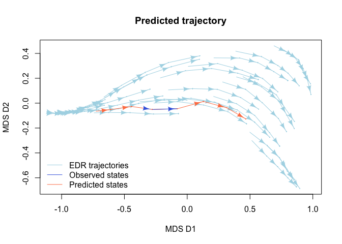
To cite ecoregime in publications use:
Sánchez-Pinillos M, Kéfi S, De Cáceres M, Dakos V (2023). “Ecological dynamic regimes: Identification, characterization, and comparison.” Ecological Monographs, e1589. https://doi.org/10.1002/ecm.1589.
Sánchez-Pinillos M, Dakos V, Kéfi S (2024). “Ecological dynamic regimes: A key concept for assessing ecological resilience.” Biological Conservation, 110409. https://doi.org/10.1016/j.biocon.2023.110409.
Sánchez-Pinillos M, Fortin M, Messier C, Kneeshaw D (2026). “Forecasting ecological trajectories from ecological dynamic regimes to improve resilience analysis.” Methods in Ecology and Evolution. https://doi.org/10.1111/2041-210x.70372.
Sánchez-Pinillos M (2023). ecoregime: Analysis of Ecological Dynamic Regimes. https://doi.org/10.5281/zenodo.7584943.
This project has received funding from the European Union’s Horizon 2020 research and innovation program under the Marie Sklodowska-Curie grant agreement No 891477 (RESET project) and the Natural Sciences and Engineering Research Council of Canada (NSERC) [DIVERSE project; funding reference ALLRP 583409-23].
These binaries (installable software) and packages are in development.
They may not be fully stable and should be used with caution. We make no claims about them.
Health stats visible at Monitor.