The hardware and bandwidth for this mirror is donated by dogado GmbH, the Webhosting and Full Service-Cloud Provider. Check out our Wordpress Tutorial.
If you wish to report a bug, or if you are interested in having us mirror your free-software or open-source project, please feel free to contact us at mirror[@]dogado.de.
The goal of drpop is to provide users doubly robust and efficient estimates of population size and the confidence intervals for a capture-recapture problem.
You can install the released version of drpop from CRAN with:
install.packages("drpop")And the development version from GitHub with:
# install.packages("devtools")
devtools::install_github("mqnjqrid/drpop")This is a basic example which shows you how to solve a common problem:
library(drpop)
#> Registered S3 methods overwritten by 'tibble':
#> method from
#> format.tbl pillar
#> print.tbl pillar
n = 1000
x = matrix(rnorm(n*3, 2, 1), nrow = n)
expit = function(xi) {
exp(sum(xi))/(1 + exp(sum(xi)))
}
y1 = unlist(apply(x, 1, function(xi) {sample(c(0, 1), 1, replace = TRUE, prob = c(1 - expit(-0.6 + 0.4*xi), expit(-0.6 + 0.4*xi)))}))
y2 = unlist(apply(x, 1, function(xi) {sample(c(0, 1), 1, replace = TRUE, prob = c(1 - expit(-0.6 + 0.3*xi), expit(-0.6 + 0.3*xi)))}))
datacrc = cbind(y1, y2, exp(x/2))[y1+y2 > 0, ]
estim <- popsize(data = datacrc, func = c("gam"), nfolds = 2, K = 2)
#> Warning: package 'dplyr' was built under R version 4.0.5
#> Loading required package: tidyr
#> Loaded gam 1.20
#> Warning in popsize_base(data, K = K, j0 = j, k0 = k, filterrows = filterrows, :
#> Plug-in variance is not well-defined. Returning variance evaluated using DR
#> estimator formula
# The population size estimates are 'n' and the standard deviations are 'sigman'
print(estim)
#> listpair model method psi sigma n sigman cin.l cin.u
#> 1 1,2 gam DR 0.820 1.015 955 31.886 893 1018
#> 2 1,2 gam PI 0.810 1.015 967 32.150 904 1030
#> 3 1,2 gam TMLE 0.822 0.921 953 29.515 895 1010
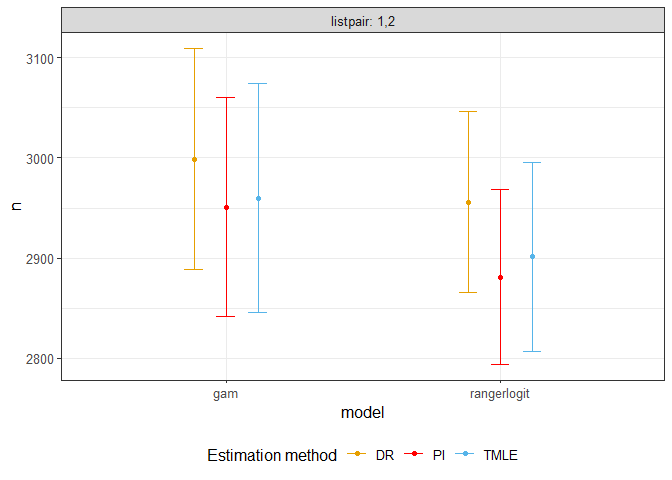
## basic example codeThe following shows the confidence interval of estimates for a toy data. Real population size is 3000.
library(drpop)

n = 3000
x = matrix(rnorm(n*3, 2,1), nrow = n)

expit = function(xi) {
  exp(sum(xi))/(1 + exp(sum(xi)))
}
y1 = unlist(apply(x, 1, function(xi) {sample(c(0, 1), 1, replace = TRUE, prob = c(1 - expit(-0.6 + 0.4*xi), expit(-0.6 + 0.4*xi)))}))
y2 = unlist(apply(x, 1, function(xi) {sample(c(0, 1), 1, replace = TRUE, prob = c(1 - expit(-0.6 + 0.3*xi), expit(-0.6 + 0.3*xi)))}))
datacrc = cbind(y1, y2, exp(x/2))[y1+y2>0,]

estim <- popsize(data = datacrc, func = c("gam", "rangerlogit"), nfolds = 2, margin = 0.01)
#> Warning in popsize_base(data, K = K, j0 = j, k0 = k, filterrows = filterrows, :
#> Plug-in variance is not well-defined. Returning variance evaluated using DR
#> estimator formula
print(estim)
#>   listpair       model method   psi sigma    n sigman cin.l cin.u
#> 1      1,2         gam     DR 0.794 1.001 2999 56.258  2889  3109
#> 2      1,2         gam     PI 0.807 1.001 2951 55.612  2842  3060
#> 3      1,2         gam   TMLE 0.805 1.059 2960 58.228  2846  3074
#> 4      1,2 rangerlogit     DR 0.806 0.764 2956 45.880  2866  3046
#> 5      1,2 rangerlogit     PI 0.827 0.764 2881 44.678  2794  2969
#> 6      1,2 rangerlogit   TMLE 0.821 0.841 2902 48.147  2807  2996
plotci(estim)
#> Warning: package 'ggplot2' was built under R version 4.0.4
#result = melt(as.data.frame(estim), variable.name = "estimator", value.name = "population_size")
#ggplot(result, aes(x = population_size - n, fill = estimator, color = estimator)) +
#  geom_density(alpha = 0.4) +
#  xlab("Bias on n")
The following shows confidence interval of estimates for toy data with a categorical covariate. Real population size is 10000.
library(drpop)
n = 10000
x = matrix(rnorm(n*3, 2, 1), nrow = n)
expit = function(xi) {
  exp(sum(xi))/(1 + exp(sum(xi)))
}
catcov = sample(c('m','f'), n, replace = TRUE, prob = c(0.45, 0.55))

y1 = unlist(apply(x, 1, function(xi) {sample(c(0, 1), 1, replace = TRUE, prob = c(1 - expit(-0.6 + 0.4*xi), expit(-0.6 + 0.4*xi)))}))
y2 = sapply(1:n, function(i) {sample(c(0, 1), 1, replace = TRUE, prob = c(1 - expit(-0.6 + 0.3*(catcov[i] == 'm') + 0.3*x[i,]), expit(-0.6 + 0.3*(catcov[i] == 'm') + 0.3*x[i,])))})
datacrc = cbind.data.frame(y1, y2, exp(x/2), catcov)[y1+y2>0,]

result = popsize_cond(data = datacrc, condvar = 'catcov')
#> Warning in popsize_base(data = datasub, K = K, filterrows = filterrows, : Plug-
#> in variance is not well-defined. Returning variance evaluated using DR estimator
#> formula

#> Warning in popsize_base(data = datasub, K = K, filterrows = filterrows, : Plug-
#> in variance is not well-defined. Returning variance evaluated using DR estimator
#> formula
fig = plotci(result)
fig + geom_hline(yintercept = table(catcov), color = "brown", linetype = "dashed")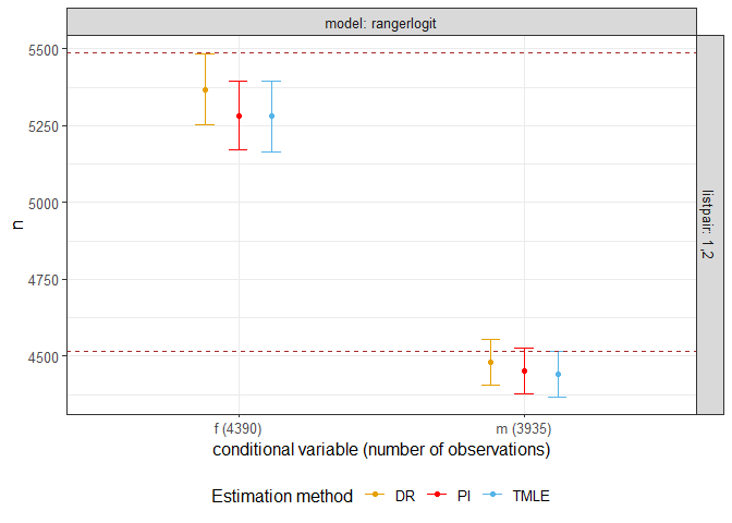
These binaries (installable software) and packages are in development.
They may not be fully stable and should be used with caution. We make no claims about them.
Health stats visible at Monitor.