

The hardware and bandwidth for this mirror is donated by dogado GmbH, the Webhosting and Full Service-Cloud Provider. Check out our Wordpress Tutorial.
If you wish to report a bug, or if you are interested in having us mirror your free-software or open-source project, please feel free to contact us at mirror[@]dogado.de.
didintrjl is an R wrapper for the Julia package DiDInt.jl, which implements intersection difference-in-differences (DID-INT), a method developed by Karim & Webb (2025). DID-INT allows for unbiased estimation of the average effect of treatment on the treated (ATT) in cases when the common causal covariates (CCC) assumption is violated.
The stable CRAN version of didintrjl can be installed via:
install.packages("didintrjl")You can install the development version of didintrjl with:
# install.packages("remotes")
remotes::install_github("ebjamieson97/didintrjl")
Since didintrjl is a wrapper for the Julia pacakage DiDInt.jl, you will need to ensure that DiDInt.jl is installed and you may need to update the Julia package itself from time to time. You can do this directly from R using the brilliant JuliaConnectoR which is the package that didintrjl uses to interface with Julia.
library(JuliaConnectoR)
juliaEval('using Pkg; Pkg.add("DiDInt")')

# Or to update:
juliaEval('using Pkg; Pkg.update("DiDInt")')didint()The didint() function returns an object with the class
DiDIntObj which has three S3 methods: print(),
summary(), and coef(). Each of these methods
have the argument level which can take either
"agg" or "sub" in order to distinguish between
aggregate results and sub-aggregate results. For example, in a staggered
adoption setting with several different treatment times, setting
level = "sub" will return information pertinent to the
distinct treatment times, whereas level = "agg" would
return the aggregated results.
# Load data
df <- read.csv("inst/extdata/merit.csv")

# Load didintrjl and run didint()
library(didintrjl)
res <- didint("coll", "state", "year", df, verbose = FALSE,
              treated_states = c(71, 58, 64, 59, 85, 57, 72, 61, 34, 88),
              treatment_times = c(1991, 1993, 1996, 1997, 1997, 1998, 1998, 1999, 2000, 2000))
#> Starting Julia ...

# Show summary of results
summary(res)
#>
#>   Model Specification: Two-way DID-INT
#>   Weighting: both
#>   Aggregation: cohort
#>   Period Length: 1 year
#>   First Period: 1989
#>   Last Period: 2000
#>   Permutations: 999
#>
#> Aggregate Results:
#>         ATT Std. Error     p-value RI p-value Jackknife SE Jackknife p-value
#>  0.04582252 0.01159691 0.007526681  0.1281281   0.01520398        0.00404305
#>
#> Subaggregate Results:
#> Treatment Time              ATT         SE    p-value   RI p-val      JK SE   JK p-val     Weight
#> --------------------------------------------------------------------------------------------------------------
#> 1991-01-01               0.0529     0.0221     0.0172     0.5245         NA         NA     0.2018
#> 1993-01-01               0.0236     0.0166     0.1554     0.6947         NA         NA     0.1915
#> 1996-01-01               0.0564     0.0242     0.0208     0.4985         NA         NA     0.0757
#> 1997-01-01               0.0711     0.0230     0.0023     0.2002     0.0257     0.0080     0.3211
#> 1998-01-01               0.0485     0.0329     0.1427     0.4715     0.0838     0.5650     0.1086
#> 1999-01-01               0.0120     0.0150     0.4235     0.8809         NA         NA     0.0355
#> 2000-01-01              -0.0331     0.0320     0.3081     0.7107     0.0966     0.7336     0.0658

# The aggregate and sub-aggregate results can also be accessed via
res$agg
#>          att         se        pval   ri_pval  jknife_se jknife_pval
#> 1 0.04582252 0.01159691 0.007526681 0.1281281 0.01520398  0.00404305
res$sub
#>        group         att         se        pval   ri_pval  jknife_se
#> 1 1991-01-01  0.05290996 0.02211803 0.017190246 0.5245245         NA
#> 2 1993-01-01  0.02359277 0.01657012 0.155433859 0.6946947         NA
#> 3 1996-01-01  0.05643511 0.02422739 0.020797631 0.4984985         NA
#> 4 1997-01-01  0.07111675 0.02296333 0.002287606 0.2002002 0.02574683
#> 5 1998-01-01  0.04854361 0.03290810 0.142653420 0.4714715 0.08378975
#> 6 1999-01-01  0.01204398 0.01497416 0.423539176 0.8808809         NA
#> 7 2000-01-01 -0.03306235 0.03203587 0.308102279 0.7107107 0.09660284
#>   jknife_pval    weights
#> 1          NA 0.20179564
#> 2          NA 0.19153484
#> 3          NA 0.07567336
#> 4 0.008012064 0.32107738
#> 5 0.564954173 0.10859342
#> 6          NA 0.03548525
#> 7 0.733597087 0.06584010didint_plot()The didint_plot() function returns an object of the
class DiDIntPlotObj which has one S3 method:
plot(). This object also stores the data used to create the
plot so that users may directly access the plotting data and create
their own customized plots. didint_plot() can produce
either parallel trends plots or event study plots.
# Generate the DiDIntPlotObj for event study plot
res_event <- didint_plot(
  "coll", "state", "year", df, event = TRUE,
  treated_states = c(71, 58, 64, 59, 85, 57, 72, 61, 34, 88),
  treatment_times = c(1991, 1993, 1996, 1997, 1997, 1998, 1998, 1999,
                      2000, 2000),
  covariates = c("asian", "black", "male")
)

plot(res_event)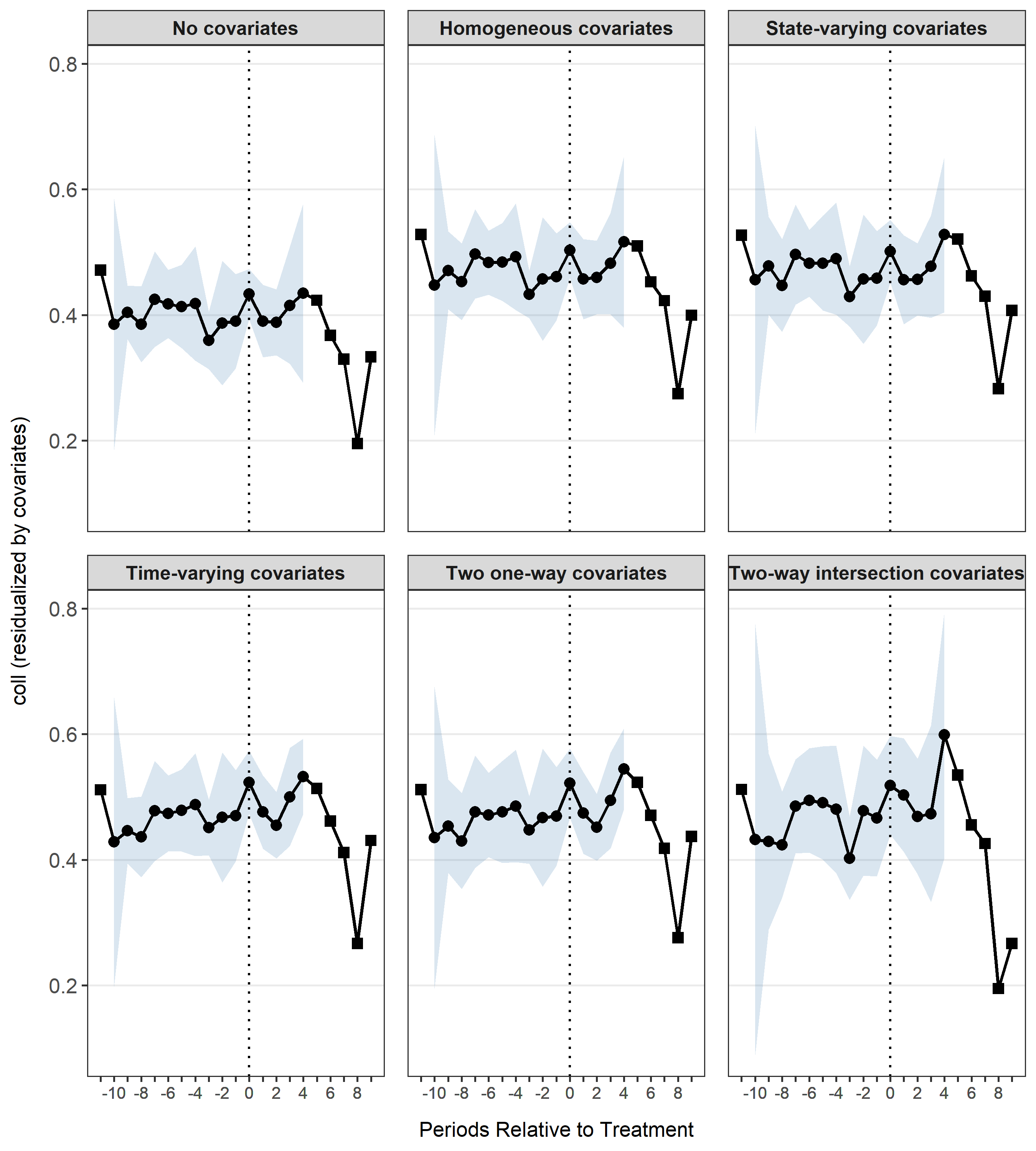
# For purposes of demonstration, it would be a bit cluttered to show the
# parallel trends for each state in the dataset, so here we will just use
# a subset
df_sub <- df[df$state %in% c(71, 58, 11, 34, 14), ]
res_parallel <- didint_plot("coll", "state", "year", df_sub,
                            treatment_times = c(1991, 1993, 2000),
                            covariates = c("asian", "black", "male"))

plot(res_parallel)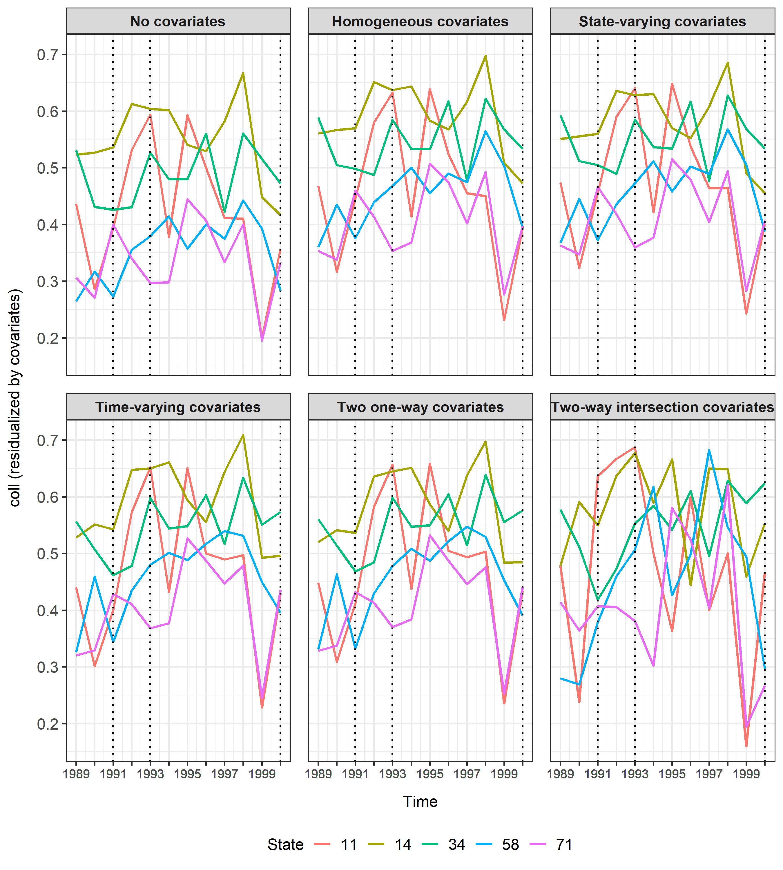
For both the event study plots and the parallel trends plots it is
possible to specify which combination of plots you would like to view
via the ccc argument.
plot(res_parallel, ccc = "state")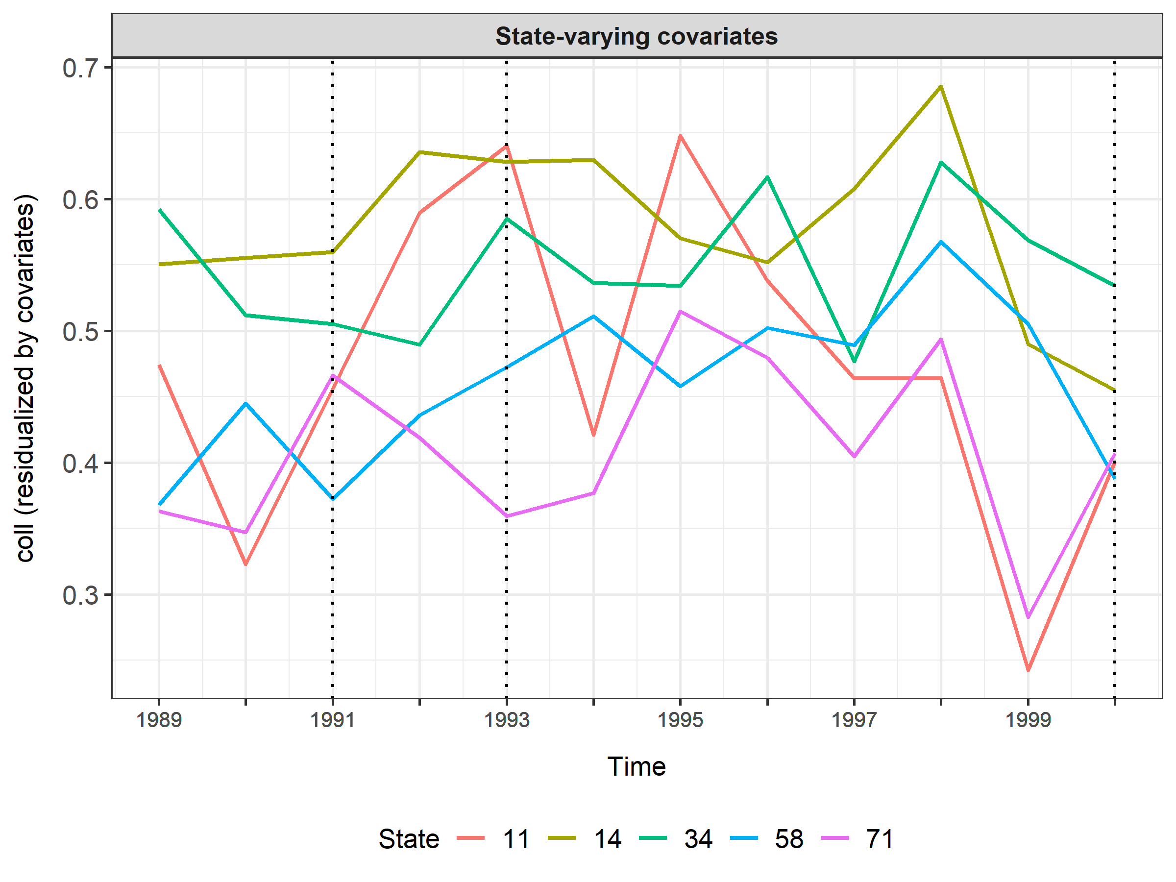
plot(res_event, ccc = c("none", "hom", "int"))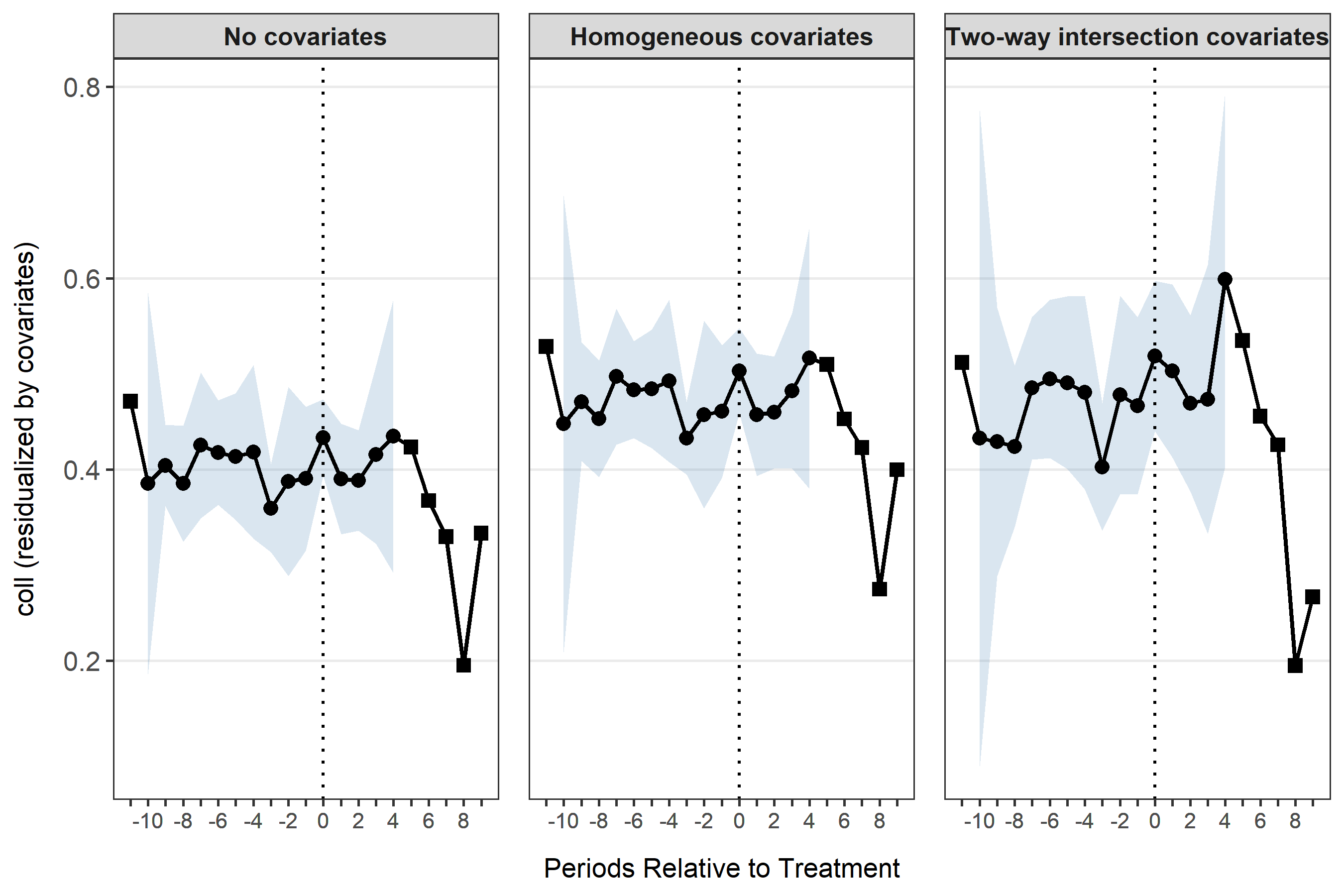
If you would like to create your own customized plots using the
plotting data, you can acccess it via
DiDIntPlotObj$data.
head(res_parallel$data)
#>   state time    lambda ccc period start_date treat_period period_length
#> 1    11 1989 0.4676477 hom      0       1989           NA        1 year
#> 2    11 1990 0.3166708 hom      1       1989           NA        1 year
#> 3    11 1991 0.4455335 hom      2       1989           NA        1 year
#> 4    11 1992 0.5796195 hom      3       1989           NA        1 year
#> 5    11 1993 0.6324456 hom      4       1989           NA        1 year
#> 6    11 1994 0.4139365 hom      5       1989           NA        1 year
head(res_event$data)
#>   ccc time_since_treatment         y         se   ci_lower  ci_upper ngroup
#> 1 hom                  -11 0.5282917 0.09643860 -0.6970768 1.7536603      2
#> 2 hom                  -10 0.4476755 0.05548662  0.2089358 0.6864151      3
#> 3 hom                   -9 0.4708055 0.02235961  0.4087253 0.5328858      5
#> 4 hom                   -8 0.4529724 0.02489070  0.3920671 0.5138777      7
#> 5 hom                   -7 0.4970207 0.03007708  0.4258997 0.5681417      8
#> 6 hom                   -6 0.4832311 0.02148627  0.4324242 0.5340381      8
#>   period_length
#> 1        1 year
#> 2        1 year
#> 3        1 year
#> 4        1 year
#> 5        1 year
#> 6        1 year
These binaries (installable software) and packages are in development.
They may not be fully stable and should be used with caution. We make no claims about them.
Health stats visible at Monitor.