The hardware and bandwidth for this mirror is donated by dogado GmbH, the Webhosting and Full Service-Cloud Provider. Check out our Wordpress Tutorial.
If you wish to report a bug, or if you are interested in having us mirror your free-software or open-source project, please feel free to contact us at mirror[@]dogado.de.

csquares

The Concise Spatial QUery And REpresentation System (c-squares) are identifiers that correspond with cells in a global grid. The system was developed by CSIRO Oceans & Atmosphere and divides the globe in rectangles of 10 by 10 degrees (longitude and latitude in WGS84). It is a hierarchical system, meaning that higher resolutions are also supported, as long as its cell size is a tenfold of 1 or 5 degrees (i.e., cells can have the following sizes in degrees: 10, 5, 1, 0.5, 0.1, etc.).

The c-squares format is a well defined exchange format for spatial raster data, it allows for light-weight text querying / aggregation and expansion to different resolutions. The csquare R package facilitates the translation of c-square code into spatial information (sf and stars) and vice versa.

For more technical information on c-squares, please consult the Wikipedia page or the CSIRO c-squares page.

Installation

Get CRAN version

install.packages("csquares")

Get development version from r-universe

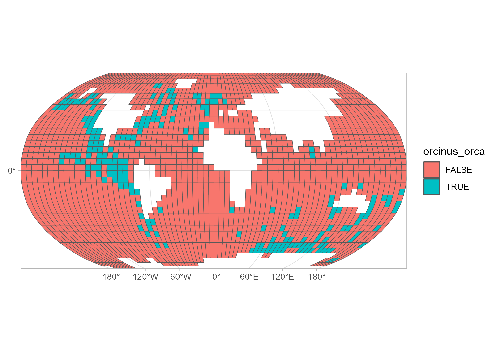
install.packages("csquares", repos = c("https://pepijn-devries.r-universe.dev", "https://cloud.r-project.org"))

Example

The example below is based on killer whale realm data extracted from the publication by Costello et al. (2017).

The orca data set itself is not provided as a simple features object, which is commonly used in R for spatial analyses. Instead, spatial information is encoded in the c-squares format. The example below shows how these codes can be decoded in a spatially explicit format which can be used for subsequent analyses.

library(csquares)
library(sf)
library(ggplot2)

## Convert the data.frame into a csquares object
orca_csq <- as_csquares(orca, csquares = "csquares")

## Convert the csquares object into a simple features object
## and transform to Robinson's projection
orca_sf <-
  orca_csq |>
  st_as_sf() |>
  st_transform(crs = "+proj=robin +lon_0=0 +x_0=0 +y_0=0")

## Make a plot of the spatial data
ggplot(orca_sf) +
  geom_sf(aes(fill = orcinus_orca)) +
  coord_sf(expand = FALSE)

The example above uses existing data with specified c-square codes. You can also create a raster with c-square codes from scratch. The example below shows how to create a 0.1 x 0.1 degrees raster for a specific bounding box.

st_bbox(c(xmin = 5.0, xmax = 5.5, ymin = 52.5, ymax = 53), crs = 4326) |>
  new_csquares(resolution = 0.1)
#> stars object with 2 dimensions and 1 attribute
#> attribute(s):
#>   csquares         
#>  Length:25         
#>  Class :character  
#>  Mode  :character  
#> dimension(s):
#>   from to offset delta refsys x/y
#> x    1  5      5   0.1 WGS 84 [x]
#> y    1  5     53  -0.1 WGS 84 [y]

References

• https://www.cmar.csiro.au/csquares/
• https://en.wikipedia.org/wiki/C-squares
• Costello, M.J. (2017); University of Auckland https://doi.org/10.17608/k6.auckland.5086654 Licence CC BY 4.0
• Costello M.J., Tsai P., Wong P.S., Cheung A.K.L, Basher Z. & Chaudhary C. (2017); “Marine biogeographic realms and species endemicity” Nature Communications 8, 1057 https://doi.org/10.1038/s41467-017-01121-2

These binaries (installable software) and packages are in development.
They may not be fully stable and should be used with caution. We make no claims about them.
Health stats visible at Monitor.