The hardware and bandwidth for this mirror is donated by dogado GmbH, the Webhosting and Full Service-Cloud Provider. Check out our Wordpress Tutorial.
If you wish to report a bug, or if you are interested in having us mirror your free-software or open-source project, please feel free to contact us at mirror[@]dogado.de.
The goal of concorR is to implement the CONCOR (CONvergence of iterated CORrelations) algorithm for positional analysis. Positional analysis divides a network into blocks based on the similarity of links between actors. CONCOR uses structural equivalence—“same ties to same others”—as its criterion for grouping nodes, and calculates this by correlating columns in the adjacency matrix. For more details on CONCOR, see the original description by Breiger, Boorman, and Arabie (1975), or Chapter 9 in Wasserman and Faust (1994).
You can install the released version of concorR from CRAN with:
install.packages("concorR")And the development version from GitHub with:
# install.packages("devtools")
devtools::install_github("ATraxLab/concorR")This is a basic example which shows a common task: using CONCOR to partition a single adjacency matrix.
library(concorR)
a <- matrix(c(0, 0, 0, 0, 1, 1, 0, 1, 0, 1, 1, 1, 0, 1, 1,
               1, 0, 1, 0, 1, 1, 0, 0, 0, 0), ncol = 5)
rownames(a) <- letters[1:5]
colnames(a) <- letters[1:5]
concor(list(a))
#>   block vertex
#> 1     1      b
#> 2     1      c
#> 3     1      d
#> 4     2      a
#> 5     2      e
Additional helper functions are included for using the
igraph package:
library(igraph)
#>
#> Attaching package: 'igraph'
#> The following objects are masked from 'package:stats':
#>
#>     decompose, spectrum
#> The following object is masked from 'package:base':
#>
#>     union

plot(graph_from_adjacency_matrix(a))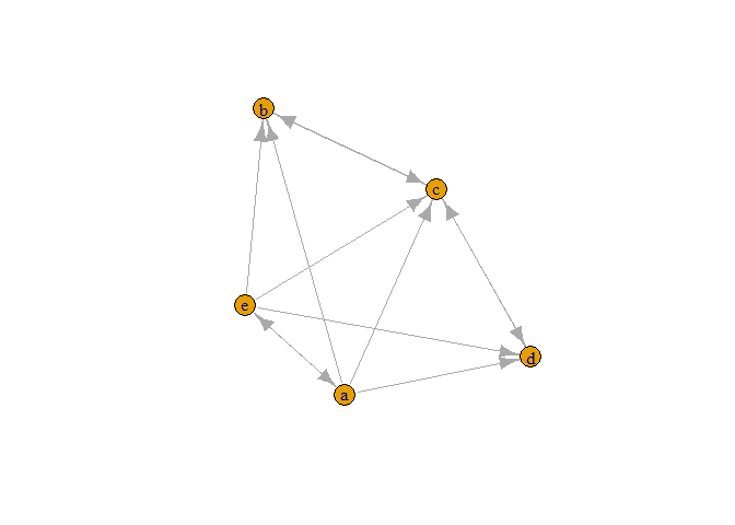
glist <- concor_make_igraph(list(a))

plot(glist[[1]], vertex.color = V(glist[[1]])$csplit1)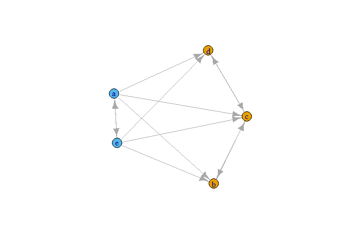
The blockmodel shows the permuted adjacency matrix, rearranged to group nodes by CONCOR partition.
bm <- make_blk(list(a), 1)[[1]]
plot_blk(bm, labels = TRUE)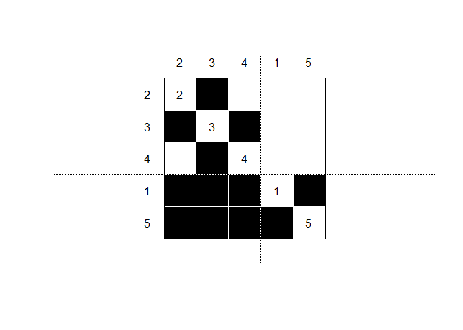
The reduced matrix represents each position as a node, and calculates links by applying a density threshold to the ties between (and within) positions.
(r_mat <- make_reduced(list(a), nsplit = 1))
#> $reduced_mat
#> $reduced_mat[[1]]
#>         Block 1 Block 2
#> Block 1       1       0
#> Block 2       1       1
#>
#>
#> $dens
#> [1] 0.6
r_igraph <- make_reduced_igraph(r_mat$reduced_mat[[1]])

plot_reduced(r_igraph)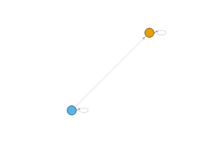
CONCOR can use multiple adjacency matrices to partition nodes based
on all relations simultaneously. The package includes
igraph data files for the Krackhardt (1987) high-tech
managers study, which gives networks for advice, friendship, and
reporting among 21 managers at a firm. (These networks were used in the
examples of Wasserman and Faust (1994).)
First, take a look at the CONCOR partitions for two splits (four positions), considering only the advice or only the friendship networks.
par(mfrow = c(1, 2))
plot_socio(krack_advice)  # plot_socio imposes some often-useful plot parameters
plot_socio(krack_friend)
par(mfrow = c(1,1))

m1 <- igraph::as_adjacency_matrix(krack_advice, sparse = FALSE)
m2 <- igraph::as_adjacency_matrix(krack_friend, sparse = FALSE)

g1 <- concor_make_igraph(list(m1), nsplit = 2)
g2 <- concor_make_igraph(list(m2), nsplit = 2)

gadv <- set_vertex_attr(krack_advice, "csplit2", value = V(g1[[1]])$csplit2)
gfrn <- set_vertex_attr(krack_friend, "csplit2", value = V(g2[[1]])$csplit2)

par(mfrow = c(1, 2))
plot_socio(gadv, nsplit = 2)
plot_socio(gfrn, nsplit = 2)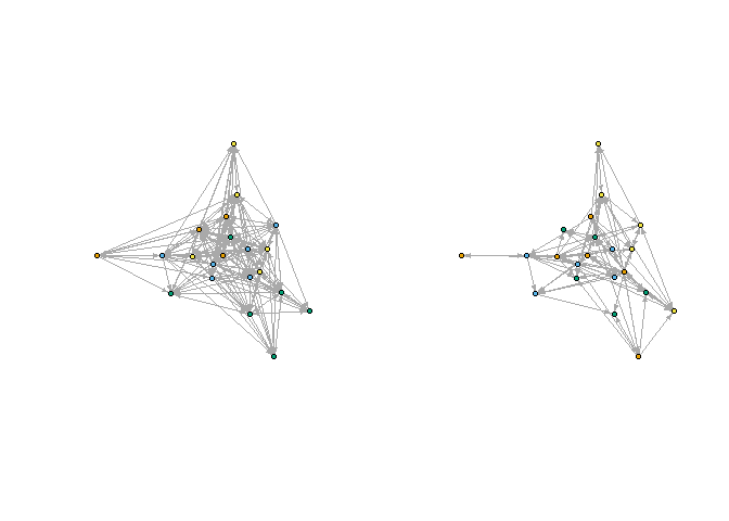
par(mfrow = c(1,1))Next, compare with the multi-relation blocking:
gboth <- concor_make_igraph(list(m1, m2), nsplit = 2)

gadv2 <- set_vertex_attr(krack_advice, "csplit2", value = V(gboth[[1]])$csplit2)
gfrn2 <- set_vertex_attr(krack_friend, "csplit2", value = V(gboth[[2]])$csplit2)

par(mfrow = c(1, 2))
plot_socio(gadv2, nsplit = 2)
plot_socio(gfrn2, nsplit = 2)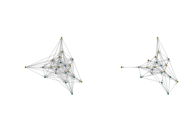
par(mfrow = c(1,1))Including information from both relations changes the block membership of several nodes.
It also affects the reduced networks, as can be seen from comparing the single-relation version:
red1 <- make_reduced(list(m1), nsplit = 2)
red2 <- make_reduced(list(m2), nsplit = 2)

gred1 <- make_reduced_igraph(red1$reduced_mat[[1]])
gred2 <- make_reduced_igraph(red2$reduced_mat[[1]])

par(mfrow = c(1, 2))
plot_reduced(gred1)
plot_reduced(gred2)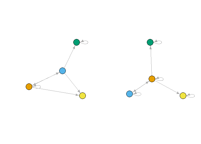
par(mfrow = c(1,1))with the multi-relation version:
redboth <- make_reduced(list(m1, m2), nsplit = 2)
gboth <- lapply(redboth$reduced_mat, make_reduced_igraph)
par(mfrow = c(1, 2))
plot_reduced(gboth[[1]])
plot_reduced(gboth[[2]])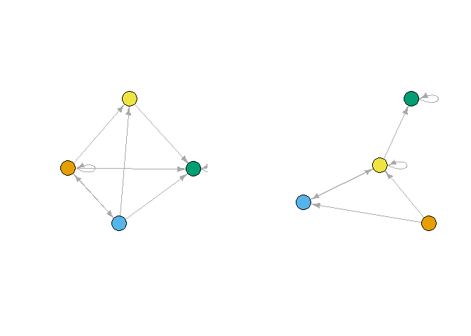
par(mfrow = c(1,1))This work was supported by National Science Foundation awards DUE-1712341 and DUE-1711017.
R. L. Breiger, S. A. Boorman, P. Arabie, An algorithm for clustering relational data with applications to social network analysis and comparison with multidimensional scaling. J. of Mathematical Psychology. 12, 328 (1975).
D. Krackhardt, Cognitive social structures. Social Networks. 9, 104 (1987).
S. Wasserman and K. Faust, Social Network Analysis: Methods and Applications (Cambridge University Press, 1994).
These binaries (installable software) and packages are in development.
They may not be fully stable and should be used with caution. We make no claims about them.
Health stats visible at Monitor.