The hardware and bandwidth for this mirror is donated by dogado GmbH, the Webhosting and Full Service-Cloud Provider. Check out our Wordpress Tutorial.
If you wish to report a bug, or if you are interested in having us mirror your free-software or open-source project, please feel free to contact us at mirror[@]dogado.de.

compositional.mle

An R package for composable maximum likelihood estimation. Solvers are first-class functions that combine via sequential chaining, parallel racing, and random restarts.

When to Use This Package

Use compositional.mle when:

Multi-modal likelihoods: Your likelihood surface has multiple local optima and you need global search strategies (simulated annealing, random restarts)
Coarse-to-fine optimization: You want to start with a rough global search and progressively refine with local methods
Comparing strategies: You’re unsure which optimizer works best and want to race them automatically
Building robust pipelines: You need reliable estimation that handles edge cases gracefully
Research/experimentation: You want to explore optimization strategies and visualize convergence

Stick with optim() when:

You have a simple, well-behaved likelihood with a single optimum
You know exactly which method works and don’t need composition

Example: Why Composition Matters

library(compositional.mle)

# A tricky bimodal likelihood
set.seed(42)
bimodal_loglike <- function(theta) {
  # Two peaks: one at theta=2, one at theta=8
  log(0.3 * dnorm(theta, 2, 0.5) + 0.7 * dnorm(theta, 8, 0.5))
}

problem <- mle_problem(
 loglike = bimodal_loglike,
  constraint = mle_constraint(support = function(theta) TRUE)
)

# Single gradient ascent gets trapped at local optimum
result_local <- gradient_ascent()(problem, theta0 = 0)

# Simulated annealing + gradient ascent finds global optimum
strategy <- sim_anneal(temp_init = 5, max_iter = 200) %>>% gradient_ascent()
result_global <- strategy(problem, theta0 = 0)

cat("Local search found:", round(result_local$theta.hat, 2),
    "(log-lik:", round(result_local$loglike, 2), ")\n")
#> Local search found: 2 (log-lik: -1.43 )
cat("Global strategy found:", round(result_global$theta.hat, 2),
    "(log-lik:", round(result_global$loglike, 2), ")\n")
#> Global strategy found: 2 (log-lik: -1.43 )

Installation

# From CRAN (when available)
install.packages("compositional.mle")

# Development version
devtools::install_github("queelius/compositional.mle")

Design Philosophy

Following SICP principles, the package provides: 1. Primitive solvers - gradient_ascent(), newton_raphson(), bfgs(), sim_anneal(), etc. 2. Composition operators - %>>% (sequential), %|% (race), with_restarts() 3. Closure property - Combining solvers yields a solver

Quick Start

# Generate sample data
set.seed(42)
x <- rnorm(100, mean = 5, sd = 2)

# Define the problem (separate from solver strategy)
problem <- mle_problem(
  loglike = function(theta) {
    if (theta[2] <= 0) return(-Inf)
    sum(dnorm(x, theta[1], theta[2], log = TRUE))
  },
  score = function(theta) {
    mu <- theta[1]; sigma <- theta[2]; n <- length(x)
    c(sum(x - mu) / sigma^2,
      -n / sigma + sum((x - mu)^2) / sigma^3)
  },
  constraint = mle_constraint(
    support = function(theta) theta[2] > 0,
    project = function(theta) c(theta[1], max(theta[2], 1e-8))
  )
)

# Simple solve
result <- gradient_ascent()(problem, theta0 = c(0, 1))
result$theta.hat
#> [1] 5.065030 2.072274

Composing Solvers

Sequential Chaining (`%>>%`)

Chain solvers for coarse-to-fine optimization:

# Grid search -> gradient ascent -> Newton-Raphson
strategy <- grid_search(lower = c(-10, 0.5), upper = c(10, 5), n = 5) %>>%
  gradient_ascent(max_iter = 50) %>>%
  newton_raphson(max_iter = 20)

result <- strategy(problem, theta0 = c(0, 1))
result$theta.hat
#>     Var1     Var2 
#> 5.065030 2.072274

Parallel Racing (`%|%`)

Race multiple methods, keep the best:

# Try multiple approaches, pick winner by log-likelihood
strategy <- gradient_ascent() %|% bfgs() %|% nelder_mead()

result <- strategy(problem, theta0 = c(0, 1))
c(result$theta.hat, loglike = result$loglike)
#>                             loglike 
#>    5.065030    2.072274 -214.758518

Random Restarts

Escape local optima with multiple starting points:

strategy <- with_restarts(
  gradient_ascent(),
  n = 10,
  sampler = uniform_sampler(c(-10, 0.5), c(10, 5))
)

result <- strategy(problem, theta0 = c(0, 1))
result$theta.hat
#> [1] 5.065030 2.072274

Visualization

Track and visualize the optimization path:

# Enable tracing
trace_cfg <- mle_trace(values = TRUE, gradients = TRUE, path = TRUE)
result <- gradient_ascent(max_iter = 50)(problem, c(0, 1), trace = trace_cfg)

# Plot convergence
plot(result, which = c("loglike", "gradient"))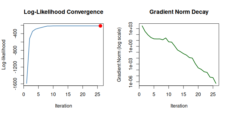

Extract trace as data frame for custom analysis:

path_df <- optimization_path(result)
head(path_df)
#>   iteration    loglike  grad_norm   theta_1  theta_2
#> 1         1 -1589.3361 2938.86063 0.0000000 1.000000
#> 2         2  -518.7066  334.47435 0.1723467 1.985036
#> 3         3  -344.5384   84.57555 0.5435804 2.913576
#> 4         4  -293.8366   30.83372 1.1733478 3.690360
#> 5         5  -271.7336   18.65296 2.1001220 4.065978
#> 6         6  -254.0618   17.83778 3.0615865 3.791049

Available Solvers

Factory	Method	Best For
`gradient_ascent()`	Steepest ascent with line search	General purpose, smooth likelihoods
`newton_raphson()`	Second-order Newton	Fast convergence near optimum
`bfgs()`	Quasi-Newton BFGS	Good balance of speed/robustness
`lbfgsb()`	L-BFGS-B with box constraints	High-dimensional, bounded parameters
`nelder_mead()`	Simplex (derivative-free)	Non-smooth or noisy likelihoods
`sim_anneal()`	Simulated annealing	Global optimization, multi-modal
`coordinate_ascent()`	One parameter at a time	Different parameter scales
`grid_search()`	Exhaustive grid	Finding starting points
`random_search()`	Random sampling	High-dimensional exploration

Function Transformers

# Stochastic gradient (mini-batching for large data)
loglike_sgd <- with_subsampling(loglike, data = x, subsample_size = 32)

# Regularization
loglike_l2 <- with_penalty(loglike, penalty_l2(), lambda = 0.1)
loglike_l1 <- with_penalty(loglike, penalty_l1(), lambda = 0.1)

Documentation

Full documentation: https://queelius.github.io/compositional.mle/
Vignettes:

License

MIT

These binaries (installable software) and packages are in development.
They may not be fully stable and should be used with caution. We make no claims about them.
Health stats visible at Monitor.