The hardware and bandwidth for this mirror is donated by dogado GmbH, the Webhosting and Full Service-Cloud Provider. Check out our Wordpress Tutorial.
If you wish to report a bug, or if you are interested in having us mirror your free-software or open-source project, please feel free to contact us at mirror[@]dogado.de.

clustringr

clustringr clusters a vector of strings into groups of small mutual “edit distance” (see stringdist), using graph algorithms. Notice it’s unsupervised, i.e., you do not need to pre-specify cluster count. Graph visualization of the results is provided.

Installation

Currently a development version is available on github.

# install.packages('devtools')
devtools::install_github('dan-reznik/clustringr')

Usage

In the example below a vector of 9 strings is clustered into 4 groups by levenshtein distance and connected components. The call to cluster_strings() returns a list w/ 3 elements, the last of which is df_clusters which associates to every input string a cluster, along with its cluster size.

library(clustringr)
s_vec <- c("alcool",
           "alcohol",
           "alcoholic",
           "brandy",
           "brandie",
           "cachaça",
           "whisky",
           "whiskie",
           "whiskers")
s_clust <- cluster_strings(s_vec # input vector
                           ,clean=T # dedup and squish
                           ,method="lv" # levenshtein
                           # use: method="dl" (dam-lev) or "osa" for opt-seq-align
                           ,max_dist=3 # max edit distance for neighbors
                           ,algo="cc" # connected components
                           # use algo="eb" for edge-betweeness
)
s_clust$df_clusters
#> # A tibble: 9 x 3
#>   cluster  size node     
#>     <int> <int> <chr>    
#> 1       1     3 alcohol  
#> 2       1     3 alcoholic
#> 3       1     3 alcool   
#> 4       2     3 whiskers 
#> 5       2     3 whiskie  
#> 6       2     3 whisky   
#> 7       3     2 brandie  
#> 8       3     2 brandy   
#> 9       4     1 cachaça

Cluster Visualization

To view a graph of the clusters, simply pass the structure returned by cluster_strings to cluster_plot:

cluster_plot(s_clust
             ,min_cluster_size=1
             # ,label_size=2.5 # size of node labels
             # ,repel=T # whether labels should be repelled
             )
#> Using `nicely` as default layout

Supplied Data Set: Don Quijote’s unique words

The clustringr package comes with quijote_words, a ~22k row data frame of the unique words (in Spanish) in Miguel de Cervantes’ “Don Quijote”. Full text can be obtained here.

Let’s sample these words into a smaller subset:

library(dplyr)
quijote_words_sampled <- clustringr::quijote_words %>%
  filter(between(freq,8,11),len>6) %>%
  pull("word")
quijote_words_sampled%>%length
#> [1] 602

Now let’s cluster these and view the results as a graph-plot, showing only those clusters with at least 3 elements:

quijote_words_sampled %>%
  cluster_strings(method="lv",max_dist=2) %>%
  cluster_plot(min_cluster_size=3)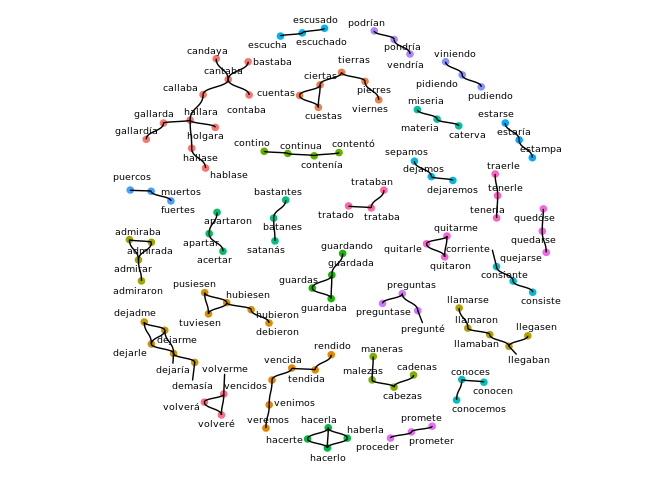

Happy clustering!

These binaries (installable software) and packages are in development.
They may not be fully stable and should be used with caution. We make no claims about them.
Health stats visible at Monitor.