The hardware and bandwidth for this mirror is donated by dogado GmbH, the Webhosting and Full Service-Cloud Provider. Check out our Wordpress Tutorial.
If you wish to report a bug, or if you are interested in having us mirror your free-software or open-source project, please feel free to contact us at mirror[@]dogado.de.

classbound

classbound is an R package for exploring and comparing classification decision boundaries. It provides a unified interface for fitting classifiers, computing 2D boundary grids, and visualizing how different models partition the feature space.

What you can do with classbound:

• Visualize decision boundaries for any R classifier
• Compare multiple classifiers side by side
• Handle high-dimensional data via 2D slicing or projection (PCA, tourr)
• View probability surfaces for classifiers that provide them
• Explore data interactively using the built-in Shiny app (explorapp())
• Integrate natively with tidymodels workflows

Full documentation: https://natydasilva.github.io/classbound/

Installation

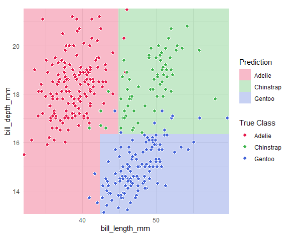
devtools::install_github("natydasilva/classbound")

Quick start

One-step wrapper

classbound() fits a model, computes its decision boundary, and plots the result in a single call.

library(classbound)
library(palmerpenguins)

penguins <- na.omit(palmerpenguins::penguins[
  ,
  c("species", "bill_length_mm", "bill_depth_mm")
])

classbound(
  data       = penguins,
  formula    = species ~ bill_length_mm + bill_depth_mm,
  classifier = rpart::rpart
)

Modular pipeline

For full control, use the three-step pipeline:

# 1. Fit
model <- fit_model(penguins, species ~ bill_length_mm + bill_depth_mm, rpart::rpart)

# 2. Compute boundary
model <- boundary_compute(model)

# 3. Plot
plot_boundary(
  model,
  obs_data   = penguins,
  x_col      = "bill_length_mm",
  y_col      = "bill_depth_mm",
  true_label = "species"
)

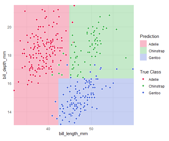
boundary_compute() returns the model with the grid attached, so you can replot with different settings without refitting.

Interactive workflow

Launch the built-in Shiny application for point-and-click exploration:

# Start with your own dataset
explorapp(data = penguins, target_col = "species")

# Or start empty and simulate/draw data
explorapp()

In explorapp() you can: - Import real data or simulate synthetic datasets - Draw classification data by hand - Fit and compare multiple classifiers simultaneously - Switch between 2D Slice and Projection views for high-dimensional data - Inject outliers and observe how boundaries shift - Inspect probability surfaces (for supported classifiers) - Export data, models, plots, and a reproduce script

Two main workflows

Interactive

Use explorapp() to:

1. Choose or create data
2. Choose models
3. Explore decision boundaries
4. Navigate, zoom, and draw
5. Compare models and export results

Programmatic

Use the core Classbound functions directly:

fit_model()
boundary_compute()
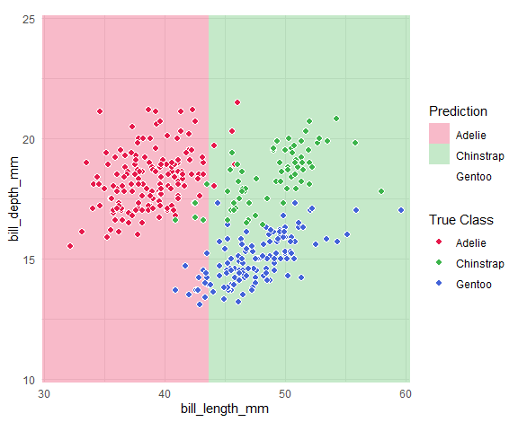
plot_boundary()

High-dimensional data

When a model is trained on more than two features, boundary_compute() supports:

• 2D Slice: two features are plotted; other features are fixed at their median/mode.

penguins3 <- na.omit(palmerpenguins::penguins[
  ,
  c("species", "bill_length_mm", "bill_depth_mm", "flipper_length_mm")
])

m3 <- fit_model(penguins3, species ~ ., rpart::rpart)
m3_slice <- boundary_compute(m3,
  feature_range = list(bill_length_mm = c(30, 60), bill_depth_mm = c(10, 25)),
  resolution = 60
)

plot_boundary(m3_slice,
  obs_data = penguins3,
  x_col = "bill_length_mm", y_col = "bill_depth_mm",
  true_label = "species"
)

• Projection: all features are combined into two projected axes (e.g., PCA).

feat_cols <- c("bill_length_mm", "bill_depth_mm", "flipper_length_mm")
pca <- prcomp(penguins3[, feat_cols], scale. = TRUE)
basis <- pca$rotation[, 1:2]

x_std <- scale(penguins3[, feat_cols], center = pca$center, scale = pca$scale)
z_mat <- x_std %*% basis

m3_proj <- boundary_compute(m3,
  feature_range = list(
    PC1 = range(z_mat[, 1]) + c(-0.5, 0.5),
    PC2 = range(z_mat[, 2]) + c(-0.5, 0.5)
  ),
  resolution = 60,
  projection = list(basis = basis, center = pca$center, scale = pca$scale)
)

plot_boundary(m3_proj,
  obs_data = penguins3,
  x_col = "PC1", y_col = "PC2", true_label = "species"
)

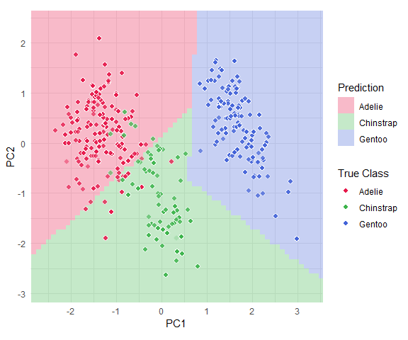
See the high-dimensional guide for a full explanation.

Multi-model comparison with tidymodels

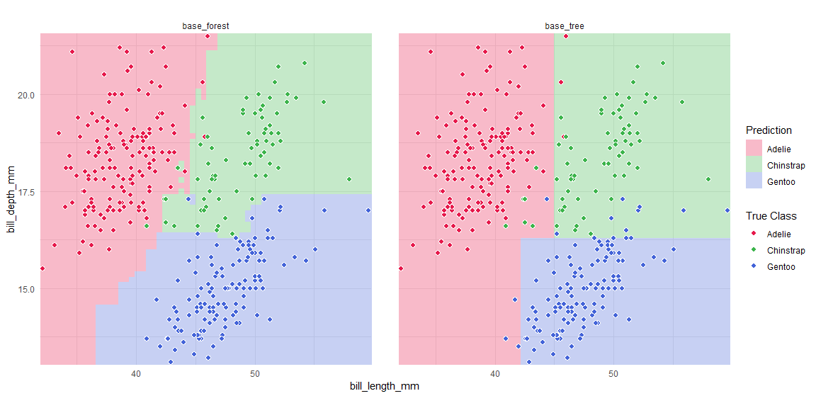
library(parsnip)
library(workflowsets)

spec_tree <- decision_tree(mode = "classification") |> set_engine("rpart")
spec_rf <- rand_forest(mode = "classification") |> set_engine("randomForest")

wf_set <- workflow_set(
  preproc = list(base = species ~ bill_length_mm + bill_depth_mm),
  models  = list(tree = spec_tree, forest = spec_rf)
)

bounds <- boundary_workflow_set(wf_set,
  data = penguins,
  response = "species", resolution = 60
)

plot_boundary(bounds,
  obs_data = penguins,
  x_col = "bill_length_mm", y_col = "bill_depth_mm",
  true_label = "species"
)

Documentation

These binaries (installable software) and packages are in development.
They may not be fully stable and should be used with caution. We make no claims about them.
Health stats visible at Monitor.