
The hardware and bandwidth for this mirror is donated by dogado GmbH, the Webhosting and Full Service-Cloud Provider. Check out our Wordpress Tutorial.
If you wish to report a bug, or if you are interested in having us mirror your free-software or open-source project, please feel free to contact us at mirror[@]dogado.de.


The {choicedata} package simplifies working with choice
data in R.
Install the released version from CRAN:
install.packages("choicedata")The package breaks choice-data modeling into a series of objects. Each object contains the information needed for the next step.
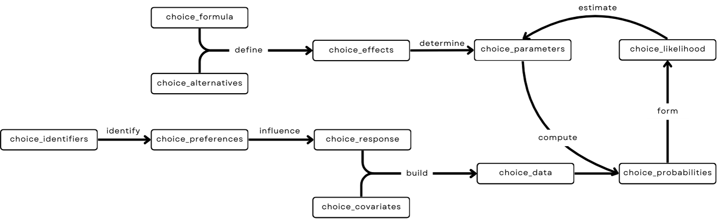
choice_formula:
the choice model formula.
choice_alternatives:
the set of choice alternatives.
choice_effects:
the choice effects, defined by choice_alternatives and
choice_formula.
choice_parameters:
the model parameters, determined by choice_effects and
estimated via choice_likelihood.
choice_identifiers:
the identifiers for deciders and choice occasions.
choice_preferences:
the choice preferences of the deciders, identified by
choice_identifiers.
choice_responses:
the choice responses, influenced by
choice_preferences.
choice_covariates:
the choice covariates.
choice_data:
the choice data, built by choice_covariates and
choice_responses.
choice_probabilities:
the choice probabilities, computed from choice_data and
choice_parameters.
choice_likelihood:
the likelihood of the choice model, formed by
choice_probabilities.
The objects are designed to be modular and can be combined in various ways to create a range of modeling workflows.
The TravelMode data set of the AER
package (Kleiber and Zeileis 2008)
contains the revealed preferences of 210 travelers choosing between air,
train, bus, and car:
library("choicedata")
data("TravelMode", package = "AER")
TravelMode$choice <- TravelMode$choice == "yes"
head(TravelMode)
#>   individual  mode choice wait vcost travel gcost income size
#> 1          1   air  FALSE   69    59    100    70     35    1
#> 2          1 train  FALSE   34    31    372    71     35    1
#> 3          1   bus  FALSE   35    25    417    70     35    1
#> 4          1   car   TRUE    0    10    180    30     35    1
#> 5          2   air  FALSE   64    58     68    68     30    2
#> 6          2 train  FALSE   44    31    354    84     30    2
We can transform the data from long (one row per choice alternative) to wide format (one row per choice occasion):
long_to_wide(
  data_frame = TravelMode,
  column_alternative = "mode",
  column_decider = "individual"
)
#> # A tibble: 210 × 20
#>    individual income  size wait_air wait_train wait_bus wait_car vcost_air
#>    <fct>       <int> <int>    <int>      <int>    <int>    <int>     <int>
#>  1 1              35     1       69         34       35        0        59
#>  2 2              30     2       64         44       53        0        58
#>  3 3              40     1       69         34       35        0       115
#>  4 4              70     3       64         44       53        0        49
#>  5 5              45     2       64         44       53        0        60
#>  6 6              20     1       69         40       35        0        59
#>  7 7              45     1       45         34       35        0       148
#>  8 8              12     1       69         34       35        0       121
#>  9 9              40     1       69         34       35        0        59
#> 10 10             70     2       69         34       35        0        58
#> # ℹ 200 more rows
#> # ℹ 12 more variables: vcost_train <int>, vcost_bus <int>, vcost_car <int>,
#> #   travel_air <int>, travel_train <int>, travel_bus <int>, travel_car <int>,
#> #   gcost_air <int>, gcost_train <int>, gcost_bus <int>, gcost_car <int>,
#> #   choice <fct>
We can construct model design matrices:
mode_data <- choice_data(
  data_frame = TravelMode,
  format = "long",
  column_choice = "choice",
  column_decider = "individual",
  column_alternative = "mode",
  column_ac_covariates = c("income", "size"),
  column_as_covariates = c("wait", "vcost", "travel", "gcost")
)

mode_effects <- choice_effects(
  choice_formula = choice_formula(
    formula = choice ~ vcost | income | wait,
    error_term = "probit"
  ),
  choice_alternatives = choice_alternatives(
    alternatives = levels(TravelMode$mode)
  ),
  choice_data = mode_data
)

mode_design <- design_matrices(mode_data, mode_effects)
mode_design[[1]] |> round()
#>       vcost income_bus income_car income_train ASC_bus ASC_car ASC_train
#> air      59          0          0            0       0       0         0
#> bus      25         35          0            0       1       0         0
#> car      10          0         35            0       0       1         0
#> train    31          0          0           35       0       0         1
#>       wait_air wait_bus wait_car wait_train
#> air         69        0        0          0
#> bus          0       35        0          0
#> car          0        0        0          0
#> train 0 0 0 34generate_choice_data() makes it straightforward to
simulate choice data. The example below simulates 200 ranking tasks with
three alternatives and recovers the data-generating parameters by
optimizing the likelihood:
library("choicedata")

set.seed(1)

sim_effects <- choice_effects(
  choice_formula = choice_formula(
    formula = choice ~ x | y + 0 | z,
    error_term = "logit"
  ),
  choice_alternatives = choice_alternatives(
    J = 3,
    alternatives = c("A", "B", "C")
  )
)

sim_parameters <- generate_choice_parameters(sim_effects)

(sim_data <- generate_choice_data(
  choice_effects = sim_effects,
  choice_identifiers = generate_choice_identifiers(N = 200),
  choice_parameters = sim_parameters,
  choice_type = "ranked"
))
#> # A tibble: 200 × 13
#>    deciderID occasionID choice       y    x_A     x_B     x_C     z_A    z_B
#>  * <chr>     <chr>      <chr>    <dbl>  <dbl>   <dbl>   <dbl>   <dbl>  <dbl>
#>  1 1         1          B      -0.621   0.487  0.738   0.576  -0.305   1.51
#>  2 2         1          A       0.594  -2.21   1.12   -0.0449 -0.0162  0.944
#>  3 3         1          C      -0.156   0.919  0.782   0.0746 -1.99    0.620
#>  4 4         1          A      -0.0538 -1.47  -0.478   0.418   1.36   -0.103
#>  5 5         1          B      -0.165  -1.38  -0.415  -0.394  -0.0593  1.10
#>  6 6         1          A       0.769  -0.253  0.697   0.557  -0.689  -0.707
#>  7 7         1          B       1.43   -0.112  0.881   0.398  -0.612   0.341
#>  8 8         1          B      -0.0392  1.98  -0.367  -1.04    0.570  -0.135
#>  9 9         1          A       0.153   0.690  0.0280 -0.743   0.189  -1.80
#> 10 10        1          C       0.291   2.17   0.476  -0.710   0.611  -0.934
#> # ℹ 190 more rows
#> # ℹ 4 more variables: z_C <dbl>, choice_A <int>, choice_B <int>, choice_C <int>

sim_likelihood <- choice_likelihood(
  choice_data = sim_data,
  choice_effects = sim_effects
)

true_vector <- switch_parameter_space(
  choice_parameters = sim_parameters,
  choice_effects = sim_effects
)

fit <- stats::optim(
  par = stats::rnorm(length(true_vector)),
  fn = function(par) {
    compute_choice_likelihood(
      choice_parameters = par,
      choice_likelihood = sim_likelihood,
      logarithm = TRUE,
      negative = TRUE
    )
  }
)

estimated_parameters <- switch_parameter_space(
  choice_parameters = fit$par,
  choice_effects = sim_effects
)

data.frame(dgp = true_vector, estimated = fit$par) |> round(2)
#>          dgp estimated
#> beta_1 -1.98     -2.36
#> beta_2  0.58      0.53
#> beta_3 -2.64     -2.83
#> beta_4  5.04      5.64
#> beta_5  1.04      1.18
#> beta_6 -2.59 -3.03{Rprobit} (Bauer et
al. 2023) provides maximum approximated composite marginal
likelihood estimation for efficient probit choice modeling.
{RprobitB} (Oelschläger
and Bauer 2025) provides Bayesian tools for estimating probit
models.
You have a question, found a bug, or want to contribute? Please file an issue on GitHub.
These binaries (installable software) and packages are in development.
They may not be fully stable and should be used with caution. We make no claims about them.
Health stats visible at Monitor.