The hardware and bandwidth for this mirror is donated by dogado GmbH, the Webhosting and Full Service-Cloud Provider. Check out our Wordpress Tutorial.
If you wish to report a bug, or if you are interested in having us mirror your free-software or open-source project, please feel free to contact us at mirror[@]dogado.de.

chaidr

chaidr is a base R implementation of the CHAID (Chi-squared Automatic Interaction Detection) and Exhaustive CHAID decision tree algorithms, as specified in the IBM SPSS Statistics Algorithms documentation (Kass 1980; Biggs, de Ville, and Suen 1991). The core fitting and prediction routines depend only on base R – visualization backends and ‘partykit’ integration are optional soft dependencies.

日本語版 README は README.ja.md を参照してください。

Features

• Standard CHAID and Exhaustive CHAID tree growing with multi-way splits.
• Predictors: nominal, ordinal (with a floating category for missing values), and continuous (automatically discretized into quantile bins).
• Responses: nominal (Pearson chi-squared test), ordinal (Goodman row-effects model), and continuous (one-way ANOVA F test).
• Frequency weights via freq, reproducing results on pre-aggregated data.
• Prediction of classes, class probabilities, and node membership with predict().
• Model inspection: node tables (chaid_table()), decision rules (chaid_rules()), and predictor importance (chaid_importance()).
• Evaluation: gains and lift analysis (chaid_gains()) and validation on holdout data (chaid_validate()).
• Visualization: base graphics plot(), ‘Graphviz’ DOT export (chaid_dot(), chaid_graphviz()), interactive ‘plotly’ trees (chaid_plotly()), and conversion to ‘partykit’ objects (chaid_as_party()).

When to use CHAID

If predictive accuracy is the only goal, modern gradient-boosting methods such as ‘XGBoost’ and ‘LightGBM’ will usually outperform CHAID. CHAID’s strengths lie elsewhere: interpretability of the results, direct connection to decision making, and statistical justification for every split. Rather than a black box, CHAID builds a single multi-way tree in which each split is backed by a significance test, which is why it remains a strong choice in consulting and marketing practice.

Typical applications:

• Survey analysis, customer-satisfaction (CS) studies, and market research
• Marketing segmentation and target selection
• Domains with strong accountability requirements, where every decision rule must be explainable
• Early-stage exploratory data analysis (EDA)

Installation

Once on CRAN, install the released version with:

install.packages("chaidr")

Until then, you can install the development version from GitHub:

# install.packages("remotes")
remotes::install_github("morimotoosamu/chaidr")

Quick start

The penguins data set (bundled with R >= 4.5) contains a mix of continuous predictors and missing values, both of which CHAID handles natively.

library(chaidr)

data(penguins)
fit <- chaid(species ~ ., data = penguins,
             control = chaid_control(min_parent = 30, min_child = 10))
print(fit)
#> CHAID decision tree (method = "chaid")
#> Response: species (categorical) 
#> Valid cases: 344 (data: 344 rows) 
#> 
#> [1] root: Adelie (44.2%), n=344 | split: flipper_len (adj.p=2.48e-63, chi2=328.5, B=714)
#>   [2] flipper_len in {<= 190}: Adelie (84.8%), n=99 | split: bill_len (adj.p=2.92e-16, chi2=78.21, B=28)
#>     [3] bill_len in {<= 40.1}: Adelie (100.0%), n=70 *
#>     [4] bill_len in {(40.1, 41.8]}: Adelie (92.3%), n=13 *
#>     [5] bill_len in {(41.8, 47.3] | > 49.3}: Chinstrap (87.5%), n=16 *
#>   [6] flipper_len in {(190, 196]}: Adelie (67.2%), n=67 | split: bill_len (adj.p=1.66e-13, chi2=58.69, B=9)
#>     [7] bill_len in {<= 44.4}: Adelie (100.0%), n=43 *
#>     [8] bill_len in {> 44.4}: Chinstrap (91.7%), n=24 *
#>   [9] flipper_len in {(196, 202]}: Chinstrap (52.6%), n=38 | split: bill_len (adj.p=2.31e-07, chi2=30.78, B=8)
#>     [10] bill_len in {<= 45.9}: Adelie (90.0%), n=20 *
#>     [11] bill_len in {> 47.3}: Chinstrap (100.0%), n=18 *
#>   [12] flipper_len in {(202, 214] | <NA>}: Gentoo (73.8%), n=61 | split: bill_dep (adj.p=9.69e-12, chi2=56.14, B=15)
#>     [13] bill_dep in {<= 16.7}: Gentoo (100.0%), n=44 *
#>     [14] bill_dep in {> 17.8 | <NA>}: Chinstrap (64.7%), n=17 *
#>   [15] flipper_len in {> 214}: Gentoo (100.0%), n=79 *

Continuous predictors such as flipper_len are discretized into quantile bins before growing, and statistically similar bins are merged back together, yielding multi-way splits. Groups containing <NA> show where missing values were merged as a floating category. Terminal nodes are marked with *.

The same tree can be plotted with base graphics (bars show the class distribution within each node):

plot(fit, main = "CHAID: penguins (species)")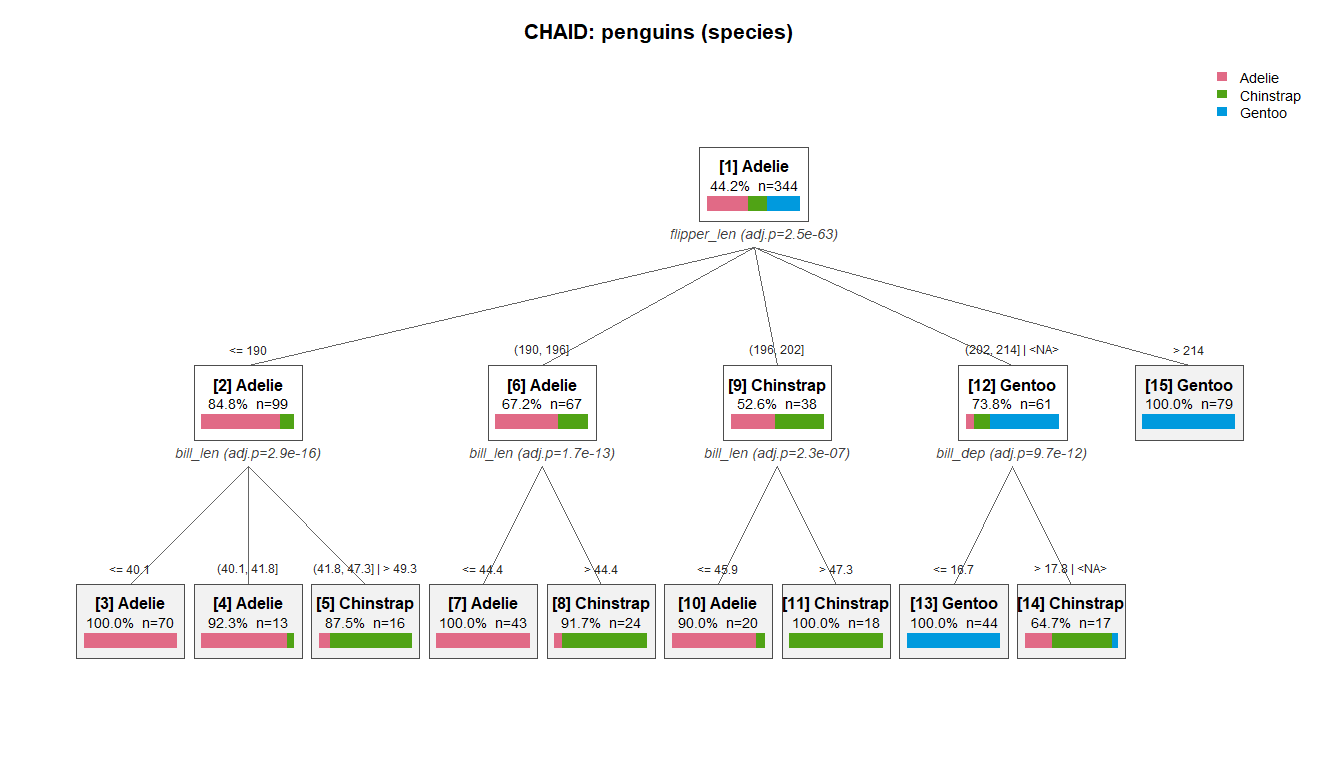

Prediction uses the standard S3 predict() interface:

pred <- predict(fit, penguins)          # class labels (factor)
mean(pred == penguins$species)          # training accuracy
#> [1] 0.9622093

round(predict(fit, head(penguins, 3), type = "prob"), 3)
#>      Adelie Chinstrap Gentoo
#> [1,]      1         0      0
#> [2,]      1         0      0
#> [3,]      1         0      0

Decision rules for every terminal node:

chaid_rules(fit)
#>    node
#> 1     3
#> 2     4
#> 3     5
#> 4     7
#> 5     8
#> 6    10
#> 7    11
#> 8    13
#> 9    14
#> 10   15
#>                                                                                                  rule
#> 1                                                             bill_len <= 40.1 and flipper_len <= 190
#> 2                                                     bill_len in (40.1, 41.8] and flipper_len <= 190
#> 3                                (bill_len in (41.8, 47.3] or bill_len > 49.3) and flipper_len <= 190
#> 4                                                      bill_len <= 44.4 and flipper_len in (190, 196]
#> 5                                                       bill_len > 44.4 and flipper_len in (190, 196]
#> 6                                                      bill_len <= 45.9 and flipper_len in (196, 202]
#> 7                                                       bill_len > 47.3 and flipper_len in (196, 202]
#> 8                          bill_dep <= 16.7 and (flipper_len in (202, 214] or flipper_len is missing)
#> 9  (bill_dep > 17.8 or bill_dep is missing) and (flipper_len in (202, 214] or flipper_len is missing)
#> 10                                                                                  flipper_len > 214

Key functions

Documentation

• vignette("chaidr") – a compact introduction (in English).
• vignette("chaidr-ja") – a detailed tutorial covering the algorithm, all option settings, evaluation, and visualization (in Japanese).

References

• Kass, G. V. (1980). An exploratory technique for investigating large quantities of categorical data. Applied Statistics, 29(2), 119–127.
• Biggs, D., de Ville, B., & Suen, E. (1991). A method of choosing multiway partitions for classification and decision trees. Journal of Applied Statistics, 18(1), 49–62.
• IBM Corp. IBM SPSS Statistics Algorithms – “CHAID and Exhaustive CHAID Algorithms”.

Acknowledgments

Development of this package was assisted by Google Gemini and Claude Code (Anthropic).

License

MIT (c) Osamu Morimoto

These binaries (installable software) and packages are in development.
They may not be fully stable and should be used with caution. We make no claims about them.
Health stats visible at Monitor.