The hardware and bandwidth for this mirror is donated by dogado GmbH, the Webhosting and Full Service-Cloud Provider. Check out our Wordpress Tutorial.
If you wish to report a bug, or if you are interested in having us mirror your free-software or open-source project, please feel free to contact us at mirror[@]dogado.de.
![]()
![]()
Package: cbbinom
0.2.0
Author: Xiurui Zhu
Modified: 2024-09-18 23:27:13
Compiled: 2024-10-16 23:21:42
The goal of cbbinom is to implement continuous
beta-binomial distribution.
You can install the released version of cbbinom from CRAN with:
install.packages("cbbinom")Alternatively, you can install the developmental version of
cbbinom from github
with:
remotes::install_github("zhuxr11/cbbinom")The continuous beta-binomial distribution spreads the standard
probability mass of beta-binomial distribution at x to an
interval [x, x + 1] in a continuous manner. This can be
validated via the following plot, where we can see that the cumulative
distribution function (CDF) of the continuous beta-binomial distribution
at x + 1 equals to that of the beta-binomial distribution
at x.
library(cbbinom)# The continuous beta-binomial CDF, shift by -1
cbbinom_plot_x <- seq(-1, 10, 0.01)
cbbinom_plot_y <- pcbbinom(
q = cbbinom_plot_x,
size = 10,
alpha = 2,
beta = 4,
ncp = -1
)
# The beta-binomial CDF
bbinom_plot_x <- seq(0L, 10L, 1L)
bbinom_plot_y <- extraDistr::pbbinom(
q = bbinom_plot_x,
size = 10L,
alpha = 2,
beta = 4
)
ggplot2::ggplot(mapping = ggplot2::aes(x = x, y = y)) +
ggplot2::geom_bar(
data = data.frame(
x = bbinom_plot_x,
y = bbinom_plot_y
),
stat = "identity"
) +
ggplot2::geom_point(
data = data.frame(
x = cbbinom_plot_x,
y = cbbinom_plot_y
)
) +
ggplot2::scale_x_continuous(
n.breaks = diff(range(cbbinom_plot_x))
) +
ggplot2::theme_bw() +
ggplot2::labs(y = "CDF(x)")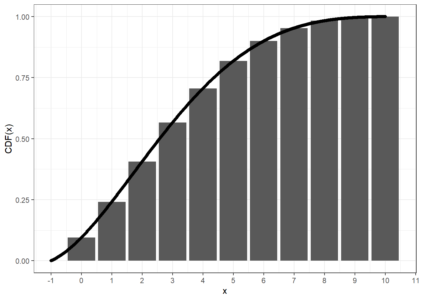
However, the central density at x + 1/2 of the
continuous beta-binomial distribution may not equal to the corresponding
probability mass at x, especially around the summit and to
the right (since alpha < beta).
# The continuous beta-binomial CDF, shift by -1/2
cbbinom_plot_x_d <- seq(-1/2, 10 + 1/2, 0.01)
cbbinom_plot_y_d <- dcbbinom(
  x = cbbinom_plot_x_d,
  size = 10,
  alpha = 2,
  beta = 4,
  ncp = -1/2
)
# The beta-binomial CDF
bbinom_plot_x <- seq(0L, 10L, 1L)
bbinom_plot_y_d <- extraDistr::dbbinom(
  x = bbinom_plot_x,
  size = 10L,
  alpha = 2,
  beta = 4
)
ggplot2::ggplot(mapping = ggplot2::aes(x = x, y = y)) +
  ggplot2::geom_bar(
    data = data.frame(
      x = bbinom_plot_x,
      y = bbinom_plot_y_d
    ),
    stat = "identity"
  ) +
  ggplot2::geom_point(
    data = data.frame(
      x = cbbinom_plot_x_d,
      y = cbbinom_plot_y_d
    )
  ) +
  ggplot2::scale_x_continuous(
    n.breaks = diff(range(bbinom_plot_x))
  ) +
  ggplot2::theme_bw() +
  ggplot2::labs(y = "PDF(x)")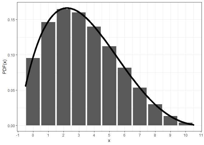
For larger sizes, you may need higher precision than double for accuracy, at the cost of computational speed.
cbbinom_plot_prec_x_p <- seq(0, 41, 0.1)
# Compute CDF at default (double) precision level
system.time(pcbbinom_plot_prec0_y <- pcbbinom(
  q = cbbinom_plot_prec_x_p,
  size = 40,
  alpha = 2,
  beta = 4,
  prec = NULL
))
#>    user  system elapsed
#> 0.03 0.00 0.03ggplot2::ggplot(data = data.frame(x = cbbinom_plot_prec_x_p,
y = pcbbinom_plot_prec0_y),
mapping = ggplot2::aes(x = x, y = y)) +
ggplot2::geom_point() +
ggplot2::theme_bw() +
ggplot2::labs(y = "CDF(x)")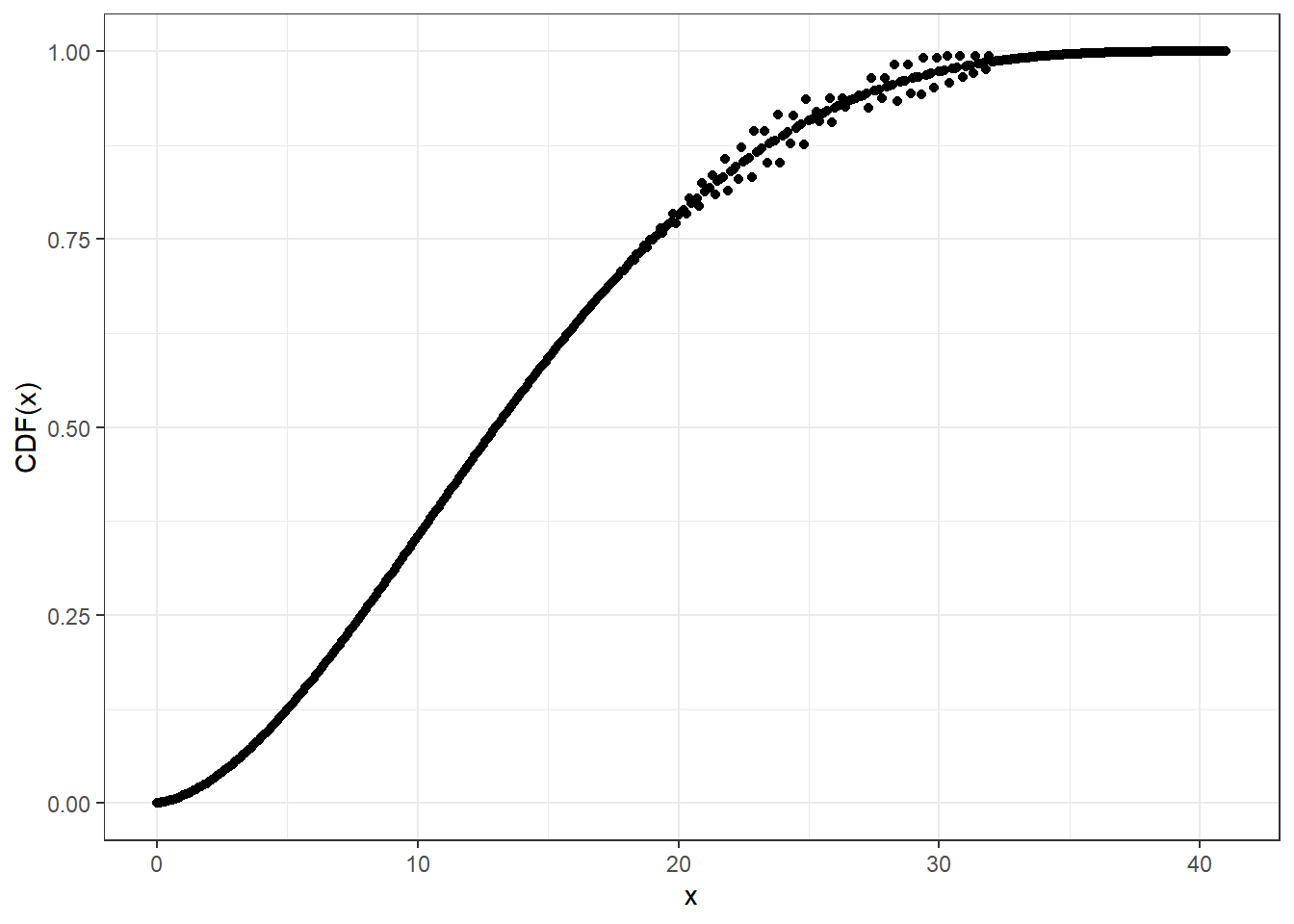
# Compute CDF at precision level 20
system.time(pcbbinom_plot_prec20_y <- pcbbinom(
  q = cbbinom_plot_prec_x_p,
  size = 40,
  alpha = 2,
  beta = 4,
  prec = 20L
))
#>    user  system elapsed
#> 1.57 0.00 1.59ggplot2::ggplot(data = data.frame(x = cbbinom_plot_prec_x_p,
y = pcbbinom_plot_prec20_y),
mapping = ggplot2::aes(x = x, y = y)) +
ggplot2::geom_point() +
ggplot2::theme_bw() +
ggplot2::labs(y = "CDF(x)")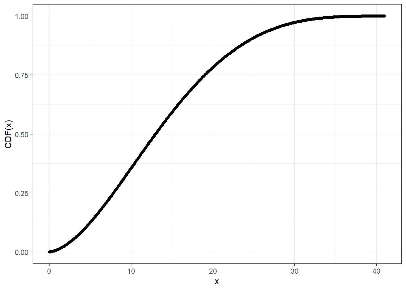
As the probability distributions in stats package,
cbbinom provides a full set of density, distribution
function, quantile function and random generation for the continuous
beta-binomial distribution.
# Density function
dcbbinom(x = 5, size = 10, alpha = 2, beta = 4)
#> [1] 0.12669
# Distribution function
(test_val <- pcbbinom(q = 5, size = 10, alpha = 2, beta = 4))
#> [1] 0.7062937# Quantile function
qcbbinom(p = test_val, size = 10, alpha = 2, beta = 4)
#> [1] 5# Random generation
set.seed(1111L)
rcbbinom(n = 10L, size = 10, alpha = 2, beta = 4)
#> [1] 3.359039 3.038286 7.110936 1.311321 5.264688 8.709005 6.720415 1.164210
#> [9] 3.868370 1.332590These functions are also available in Rcpp as
cbbinom::cpp_*cbbinom(), when using
[[Rcpp::depends(cbbinom)]] and
#include <cbbinom.h>.
For mathematical details, please check the details section of
?cbbinom.
Rcpp
implementation of stats::uniroot()As a bonus, cbbinom also exports an Rcpp
implementation of stats::uniroot() function, which may come
in handy to solve equations, especially the monotonic ones used in
quantile functions. Here is an example to calculate qnorm
from pnorm in Rcpp.
#include <iostream>
#include "cbbinom.h"
using namespace cbbinom;

// Define a functor as pnorm() - p
class PnormEqn: public UnirootEqn
{
private:
  double mu;
  double sd;
  double p;
public:
  PnormEqn(const double mu_, const double sd_, const double p_):
    mu(mu_), sd(sd_), p(p_) {}
  double operator () (const double& x) const override {
    return R::pnorm(x, this->mu, this->sd, true, false) - this->p;
  }
};

// Compute quantiles
int main() {
  double p = 0.975;  // Quantile
  PnormEqn eqn_obj(0.0, 1.0, 0.975);
  double tol = 1e-6;
  int max_iter = 10000;
  double q = cbbinom::cpp_uniroot(-1000.0, 1000.0, -p, 1.0 - p, &eqn_obj, &tol, &max_iter);
  std::cout << "Quantile at " << p << "is: " << q << std::endl;
  return 0;
}
These binaries (installable software) and packages are in development.
They may not be fully stable and should be used with caution. We make no claims about them.
Health stats visible at Monitor.