
The hardware and bandwidth for this mirror is donated by dogado GmbH, the Webhosting and Full Service-Cloud Provider. Check out our Wordpress Tutorial.
If you wish to report a bug, or if you are interested in having us mirror your free-software or open-source project, please feel free to contact us at mirror[@]dogado.de.
The inspiration for {card} was to create useful
functions and analytical approaches in computational neurocardiology,
with a on electrocardiography and epidemiology.
The areas of focus of this package are the following:
You can install the released version of {card} from CRAN with:
install.packages("card")And the development version from GitHub with:
# install.packages("devtools")
devtools::install_github("shah-in-boots/card")The intent for card is to assist in the analysis of
cardiovascular and epidemiological data, with a focus on
cardiac-specific datasets and data types.
library(card)# ECG data
data("twins")
head(twins)
#> # A tibble: 6 × 23
#> # Groups: patid, hour [6]
#> patid age bmi race smoking hptn dm chf prevchd med_beta_blockers
#> <dbl> <dbl> <dbl> <fct> <fct> <fct> <fct> <fct> <fct> <fct>
#> 1 1 49 27.4 0 1 1 0 0 0 0
#> 2 1 49 27.4 0 1 1 0 0 0 0
#> 3 1 49 27.4 0 1 1 0 0 0 0
#> 4 1 49 27.4 0 1 1 0 0 0 0
#> 5 1 49 27.4 0 1 1 0 0 0 0
#> 6 1 49 27.4 0 1 1 0 0 0 0
#> # ℹ 13 more variables: med_antidepr <fct>, beck_total <dbl>, sad_bin <fct>,
#> # sad_cat <fct>, PETdiff_2 <fct>, dyxtime <dttm>, date <date>, hour <dbl>,
#> # rDYX <dbl>, sDYX <dbl>, HR <dbl>, CP <dbl>, zip <chr>
# Outcomes data
data("stress")
head(stress)
#> # A tibble: 6 × 11
#> id start stop head_ache_date_1 head_ache_date_2 head_ache_date_3
#> <dbl> <date> <date> <date> <date> <date>
#> 1 123 2014-08-26 2016-12-08 2016-12-08 NA NA
#> 2 117 2014-08-12 2016-10-30 2016-10-30 NA NA
#> 3 145 2014-10-22 2016-07-31 2016-06-01 2016-07-31 NA
#> 4 144 2014-10-21 2017-03-24 2015-02-12 NA NA
#> 5 204 2015-03-16 2015-04-03 NA NA NA
#> 6 283 2015-10-12 2016-01-19 NA NA NA
#> # ℹ 5 more variables: heart_ache_date_1 <date>, heart_ache_date_2 <date>,
#> # heart_ache_date_3 <date>, death <dbl>, broken_heart <dbl>
# VCG data
data("geh")
head(geh)
#> # A tibble: 6 × 70
#> pid hhp_id age sex age_cat systolic_bp_first systolic_bp_second
#> <dbl> <dbl> <dbl> <fct> <fct> <dbl> <dbl>
#> 1 200481 220946 42 0 0 162 165
#> 2 200489 224643 62 1 1 133 128
#> 3 200495 224845 84 0 2 100 99
#> 4 200052 222917 65 0 2 139 141
#> 5 200517 220638 64 1 1 166 163
#> 6 200623 224862 57 0 1 151 144
#> # ℹ 63 more variables: systolic_bp_third <dbl>, diastolic_bp_first <dbl>,
#> # diastolic_bp_second <dbl>, diastolic_bp_third <dbl>,
#> # pulse_rate_first <dbl>, pulse_rate_second <dbl>, height_cm <dbl>,
#> # weight_kg <dbl>, waist_cm <dbl>, dia_trt_allopdrug <hvn_lbll>,
#> # hbp_trt_allopdrug <hvn_lbll>, hyp_trt_allopdrug <hvn_lbll>,
#> # lab_hba1c <dbl>, lab_fasting_bg <dbl>, lab_fasting_insulin <dbl>,
#> # lab_tchol <dbl>, lab_ldlchol <dbl>, lab_hdlchol <dbl>, lab_triglyc <dbl>, …This modeling algorithm requires only base R, which
allows internal flexibility for modeling heuristics and improved
efficiency. For the user, it also allows standard modeling
tools/approaches, and a flexible user interface that accounts for
individual/population analysis and single/multiple component
analysis.
There are other cosinor models available in R, however
they do not allow for simple multiple-component or individual/population
analysis in a method that is tidy (for both tidyverse and
tidymodels approaches).
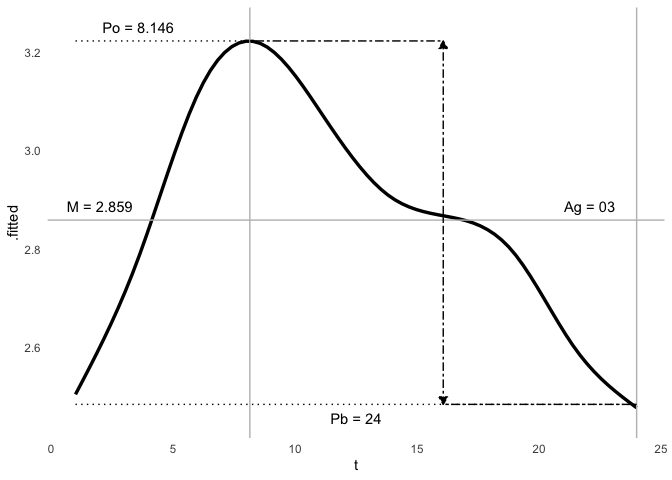
m <- cosinor(rDYX ~ hour, twins, tau = c(24, 12))
summary(m)
#> Individual Cosinor Model
#> ------------------------------------------
#> Call:
#> cosinor(formula = rDYX ~ M + A1 * cos(2*pi*hour/24 + phi1) + A2 * cos(2*pi*hour/12 + phi2)
#>
#> Period(s): 24, 12
#>
#> Residuals:
#>     Min.  1st Qu.   Median     Mean  3rd Qu.     Max.
#> -3.00770 -0.52024 -0.03247  0.00000  0.48753  4.88552
#>
#> Coefficients:
#>         Estimate  Std. Error
#> mesor  2.8586510 0.006062639
#> amp1   0.2964114 0.008702368
#> amp2   0.1302012 0.008542526
#> phi1  -2.6542757 0.028911445
#> phi2  -3.6636921 0.065235427
ggcosinor(m)
#> This is a harmonic multiple-component cosinor object. The orthophase, bathyphase, and global amplitude were calculated.
#> Warning in regularize.values(x, y, ties, missing(ties)): collapsing to unique
#> 'x' values
#> `geom_smooth()` using formula = 'y ~ s(x, bs = "cs")'
head(augment(m))
#> # A tibble: 6 × 8
#>       y     t     x1        x2        z1        z2 .fitted .resid
#>   <dbl> <dbl>  <dbl>     <dbl>     <dbl>     <dbl>   <dbl>  <dbl>
#> 1  2.63     8 -0.5   -5.00e- 1  8.66e- 1 -8.66e- 1    3.22 -0.592
#> 2  2.42     9 -0.707 -1.84e-16  7.07e- 1 -1   e+ 0    3.21 -0.787
#> 3  1.81    10 -0.866  5   e- 1  5   e- 1 -8.66e- 1    3.15 -1.34
#> 4  2.01    11 -0.966  8.66e- 1  2.59e- 1 -5.00e- 1    3.08 -1.07
#> 5  1.63    12 -1      1   e+ 0  1.22e-16 -2.45e-16    3.01 -1.38
#> 6  1.95    13 -0.966  8.66e- 1 -2.59e- 1  5   e- 1    2.95 -0.996
These binaries (installable software) and packages are in development.
They may not be fully stable and should be used with caution. We make no claims about them.
Health stats visible at Monitor.