The hardware and bandwidth for this mirror is donated by dogado GmbH, the Webhosting and Full Service-Cloud Provider. Check out our Wordpress Tutorial.
If you wish to report a bug, or if you are interested in having us mirror your free-software or open-source project, please feel free to contact us at mirror[@]dogado.de.
![]()
![]()
The bregr package revolutionizes batch regression modeling in R, enabling you to run hundreds of models simultaneously with a clean, intuitive workflow. Designed for both univariate and multivariate analyses, it delivers tidy-formatted results and publication-ready visualizations, transforming cumbersome statistical workflows into efficient pipelines.
tidyverse for seamless downstream analysis.|>).Batch regression streamlines analyses where:
A simplified overview of batch regression modeling is given below for illustration:

You can install the stable version of bregr from CRAN with:
install.packages("bregr")Alternatively, install the development version from r-universe with:
install.packages('bregr', repos = c('https://wanglabcsu.r-universe.dev', 'https://cloud.r-project.org'))or from GitHub with:
#install.packages("remotes")
remotes::install_github("WangLabCSU/bregr")Load package(s):
library(bregr)
#> Welcome to 'bregr' package!
#> =======================================================================
#> You are using bregr version 1.3.2
#>
#> Project home : https://github.com/WangLabCSU/bregr
#> Documentation: https://wanglabcsu.github.io/bregr/
#> Cite as      : https://doi.org/10.1002/mdr2.70028
#>   Wang, S., Peng, Y., Shu, C., Wang, C., Yang, Y., Zhao, Y., Cui, Y., Hu, D. and Zhou, J.-G. (2025),
#>   bregr: An R Package for Streamlined Batch Processing and Visualization of Biomedical Regression Models. Med Research.
#> =======================================================================
#>
Load data:
lung <- survival::lung |>
  dplyr::filter(ph.ecog != 3)
lung$ph.ecog <- factor(lung$ph.ecog)
bregr is designed and implemented following Tidy design principles and Tidyverse style guide, making it intuitive and user-friendly.
Define and construct batch models:
mds <- breg(lung) |> # Init breg object
  br_set_y(c("time", "status")) |> # Survival outcomes
  br_set_x(colnames(lung)[6:10]) |> # Focal predictors
  br_set_x2(c("age", "sex")) |> # Controls
  br_set_model("coxph") |> # Cox Proportional Hazards
  br_run() # Execute models
#> exponentiate estimates of model(s) constructed from coxph method at defaultmds <- br_pipeline(
lung,
y = c("time", "status"),
x = colnames(lung)[6:10],
x2 = c("age", "sex"),
method = "coxph"
)Run in parallel:
mds_p <- br_pipeline(
  lung,
  y = c("time", "status"),
  x = colnames(lung)[6:10],
  x2 = c("age", "sex"),
  method = "coxph",
  n_workers = 3
)
#> exponentiate estimates of model(s) constructed from coxph method at default
#> ■■■■■■■                           20% | ETA: 13s
#>
#> ■■■■■■■■■■■■■■■■■■■■■■■■■■■■■■■ 100% | ETA: 0sall.equal(mds, mds_p)
#> [1] TRUETwo global options have been introduced to control whether models are
saved as local files (bregr.save_model, default is
FALSE) and where they should be saved
(bregr.path, default uses a temporary path).
Use br_get_*() function family to access attributes and
data of result breg object.
br_get_models(mds) # Raw model objects
#> $ph.ecog
#> Call:
#> survival::coxph(formula = survival::Surv(time, status) ~ ph.ecog +
#>     age + sex, data = data)
#>
#>               coef exp(coef)  se(coef)      z        p
#> ph.ecog1  0.409836  1.506571  0.199606  2.053  0.04005
#> ph.ecog2  0.902321  2.465318  0.228092  3.956 7.62e-05
#> age       0.010777  1.010836  0.009312  1.157  0.24713
#> sex      -0.545631  0.579476  0.168229 -3.243  0.00118
#>
#> Likelihood ratio test=28.94  on 4 df, p=8.052e-06
#> n= 226, number of events= 163
#>
#> $ph.karno
#> Call:
#> survival::coxph(formula = survival::Surv(time, status) ~ ph.karno +
#>     age + sex, data = data)
#>
#>               coef exp(coef)  se(coef)      z       p
#> ph.karno -0.012238  0.987837  0.005946 -2.058 0.03957
#> age       0.012615  1.012695  0.009462  1.333 0.18244
#> sex      -0.485116  0.615626  0.168170 -2.885 0.00392
#>
#> Likelihood ratio test=17.21  on 3 df, p=0.0006413
#> n= 225, number of events= 162
#>    (1 observation deleted due to missingness)
#>
#> $pat.karno
#> Call:
#> survival::coxph(formula = survival::Surv(time, status) ~ pat.karno +
#>     age + sex, data = data)
#>
#>                coef exp(coef)  se(coef)      z        p
#> pat.karno -0.018736  0.981439  0.005676 -3.301 0.000964
#> age        0.011672  1.011740  0.009381  1.244 0.213436
#> sex       -0.505205  0.603382  0.169452 -2.981 0.002869
#>
#> Likelihood ratio test=23.07  on 3 df, p=3.896e-05
#> n= 223, number of events= 160
#>    (3 observations deleted due to missingness)
#>
#> $meal.cal
#> Call:
#> survival::coxph(formula = survival::Surv(time, status) ~ meal.cal +
#>     age + sex, data = data)
#>
#>                coef  exp(coef)   se(coef)      z      p
#> meal.cal -0.0001535  0.9998465  0.0002409 -0.637 0.5239
#> age       0.0149375  1.0150496  0.0106016  1.409 0.1588
#> sex      -0.4775830  0.6202808  0.1914559 -2.494 0.0126
#>
#> Likelihood ratio test=10.1  on 3 df, p=0.0177
#> n= 179, number of events= 132
#>    (47 observations deleted due to missingness)
#>
#> $wt.loss
#> Call:
#> survival::coxph(formula = survival::Surv(time, status) ~ wt.loss +
#>     age + sex, data = data)
#>
#>               coef  exp(coef)   se(coef)      z       p
#> wt.loss -0.0002676  0.9997324  0.0062908 -0.043 0.96607
#> age      0.0199314  1.0201314  0.0097178  2.051 0.04027
#> sex     -0.5067253  0.6024652  0.1748697 -2.898 0.00376
#>
#> Likelihood ratio test=13.87  on 3 df, p=0.003086
#> n= 212, number of events= 150
#>    (14 observations deleted due to missingness)
br_get_results(mds) # Comprehensive estimates
#> # A tibble: 17 × 21
#>    Focal_variable term      variable  var_label var_class var_type   var_nlevels
#>    <chr>          <chr>     <chr>     <chr>     <chr>     <chr>            <int>
#>  1 ph.ecog        ph.ecog0  ph.ecog   ph.ecog   factor    categoric…           3
#>  2 ph.ecog        ph.ecog1  ph.ecog   ph.ecog   factor    categoric…           3
#>  3 ph.ecog        ph.ecog2  ph.ecog   ph.ecog   factor    categoric…           3
#>  4 ph.ecog        age       age       age       numeric   continuous          NA
#>  5 ph.ecog        sex       sex       sex       numeric   continuous          NA
#>  6 ph.karno       ph.karno  ph.karno  ph.karno  numeric   continuous          NA
#>  7 ph.karno       age       age       age       numeric   continuous          NA
#>  8 ph.karno       sex       sex       sex       numeric   continuous          NA
#>  9 pat.karno      pat.karno pat.karno pat.karno numeric   continuous          NA
#> 10 pat.karno      age       age       age       numeric   continuous          NA
#> 11 pat.karno      sex       sex       sex       numeric   continuous          NA
#> 12 meal.cal       meal.cal  meal.cal  meal.cal  numeric   continuous          NA
#> 13 meal.cal       age       age       age       numeric   continuous          NA
#> 14 meal.cal       sex       sex       sex       numeric   continuous          NA
#> 15 wt.loss        wt.loss   wt.loss   wt.loss   numeric   continuous          NA
#> 16 wt.loss        age       age       age       numeric   continuous          NA
#> 17 wt.loss        sex       sex       sex       numeric   continuous          NA
#> # ℹ 14 more variables: contrasts <chr>, contrasts_type <chr>,
#> #   reference_row <lgl>, label <chr>, n_obs <dbl>, n_ind <dbl>, n_event <dbl>,
#> #   exposure <dbl>, estimate <dbl>, std.error <dbl>, statistic <dbl>,
#> #   p.value <dbl>, conf.low <dbl>, conf.high <dbl>
br_get_results(mds, tidy = TRUE) # Tidy-formatted coefficients
#> # A tibble: 16 × 8
#>    Focal_variable term   estimate std.error statistic p.value conf.low conf.high
#>    <chr>          <chr>     <dbl>     <dbl>     <dbl>   <dbl>    <dbl>     <dbl>
#>  1 ph.ecog        ph.ec…    1.51   0.200       2.05   4.01e-2    1.02      2.23
#>  2 ph.ecog        ph.ec…    2.47   0.228       3.96   7.62e-5    1.58      3.86
#>  3 ph.ecog        age       1.01   0.00931     1.16   2.47e-1    0.993     1.03
#>  4 ph.ecog        sex       0.579  0.168      -3.24   1.18e-3    0.417     0.806
#>  5 ph.karno       ph.ka…    0.988  0.00595    -2.06   3.96e-2    0.976     0.999
#>  6 ph.karno       age       1.01   0.00946     1.33   1.82e-1    0.994     1.03
#>  7 ph.karno       sex       0.616  0.168      -2.88   3.92e-3    0.443     0.856
#>  8 pat.karno      pat.k…    0.981  0.00568    -3.30   9.64e-4    0.971     0.992
#>  9 pat.karno      age       1.01   0.00938     1.24   2.13e-1    0.993     1.03
#> 10 pat.karno      sex       0.603  0.169      -2.98   2.87e-3    0.433     0.841
#> 11 meal.cal       meal.…    1.000  0.000241   -0.637  5.24e-1    0.999     1.00
#> 12 meal.cal       age       1.02   0.0106      1.41   1.59e-1    0.994     1.04
#> 13 meal.cal       sex       0.620  0.191      -2.49   1.26e-2    0.426     0.903
#> 14 wt.loss        wt.lo…    1.000  0.00629    -0.0425 9.66e-1    0.987     1.01
#> 15 wt.loss        age       1.02   0.00972     2.05   4.03e-2    1.00      1.04
#> 16 wt.loss sex 0.602 0.175 -2.90 3.76e-3 0.428 0.849bregr mainly provides br_show_forest() for plotting data
table of modeling results.
br_show_forest(mds)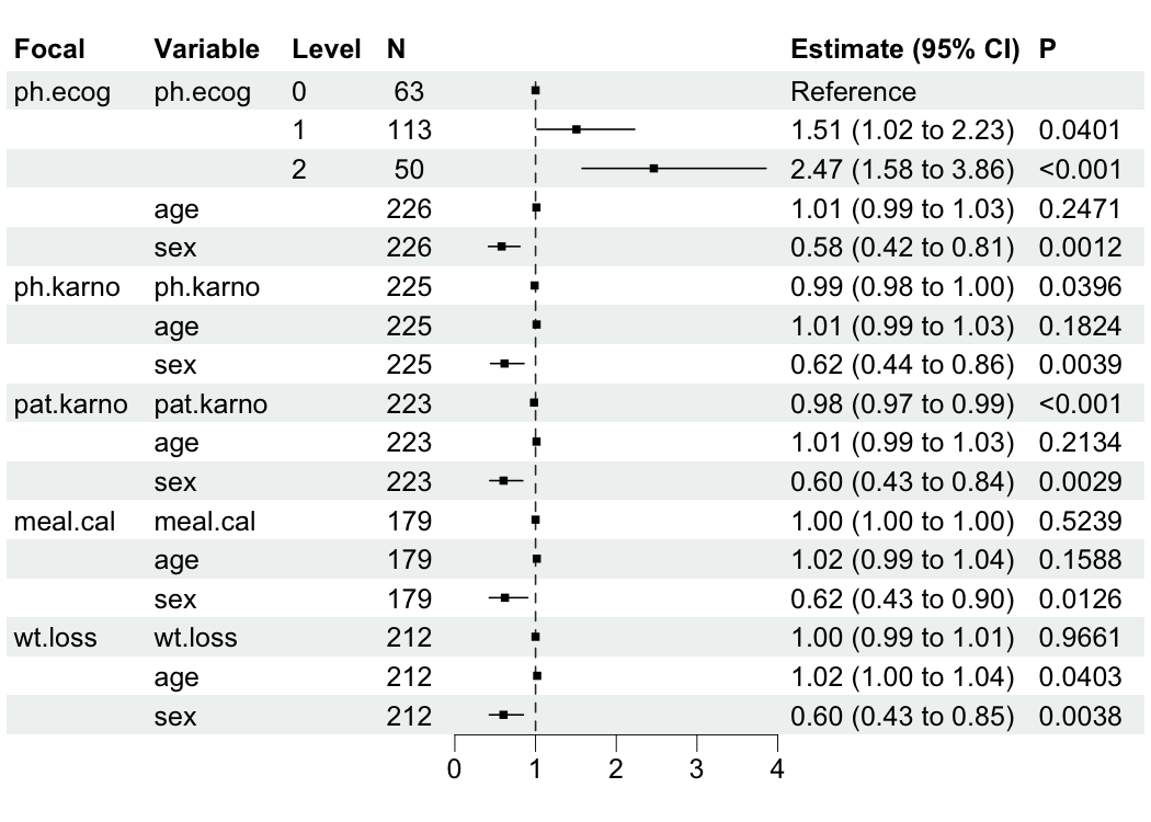
We can tune the plot to only keep focal variables and adjust the limits of x axis.
br_show_forest(
  mds,
  rm_controls = TRUE, # Focus on focal predictors
  xlim = c(0, 3), # Custom axis scaling
  #   Use x_trans = "log" to transform the axis
  #   Use log_first = TRUE to transform both
  #       the axis and estimate table
  drop = 1 # Remove redundant columns
)
We also provide some interfaces from other packages for plotting
constructed model(s), e.g., br_show_forest_ggstats(),
br_show_forest_ggstatsplot(),
br_show_fitted_line(), and
br_show_fitted_line_2d().
A common analysis task is to compare how predictor effects change
when modeled individually (univariate) versus together (multivariate).
The br_compare_models() function builds both types of
models and displays them side-by-side:
# Compare univariate and multivariate models
comparison <- br_compare_models(
  lung,
  y = c("time", "status"),
  x = c("ph.ecog", "ph.karno", "pat.karno"),
  x2 = c("age", "sex"),
  method = "coxph"
)
#> Building univariate models...
#> exponentiate estimates of model(s) constructed from coxph method at default
#> Building multivariate model...
#> exponentiate estimates of model(s) constructed from coxph method at default

# Show forest plot with both models
br_show_forest_comparison(comparison)
This allows you to see how adjusting for other predictors affects the estimates for each variable.
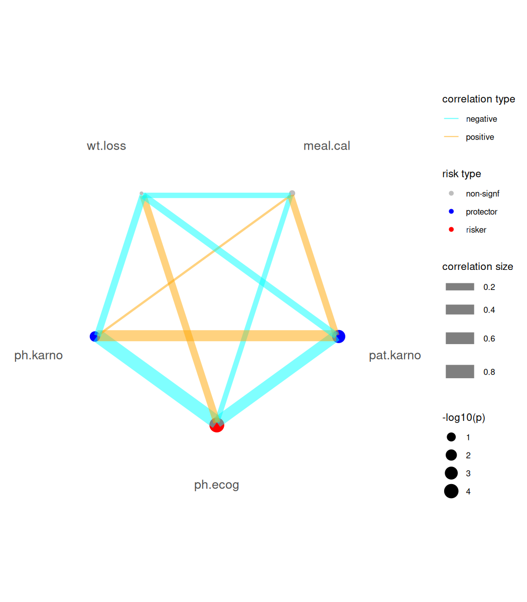
For Cox-PH modeling results (focal variables must be continuous type), we provide a risk network plotting function.
mds2 <- br_pipeline(
  survival::lung,
  y = c("time", "status"),
  x = colnames(survival::lung)[6:10],
  x2 = c("age", "sex"),
  method = "coxph"
)
#> exponentiate estimates of model(s) constructed from coxph method at defaultbr_show_risk_network(mds2)
#> please note only continuous focal terms analyzed and visualized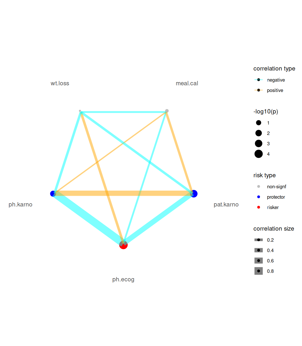
For Cox-PH models, you can generate model predictions (risk scores) and create survival curves grouped by these scores:
# Generate model predictions
scores <- br_predict(mds2, idx = "ph.ecog")
#> `type` is not specified, use lp for the model
#> Warning: some predictions are NA, consider checking your data for missing
#> values
head(scores)
#>          1          2          3          4          5          6
#>  0.3692998 -0.1608293 -0.2936304  0.1811648 -0.2493634  0.3692998
# Create survival curves based on model scores
br_show_survival_curves(
mds2,
idx = "ph.ecog",
n_groups = 3,
title = "Survival Curves by 'ph.ecog' Model Risk Score"
)
#> Warning: some predictions are NA, consider checking your data for missing
#> values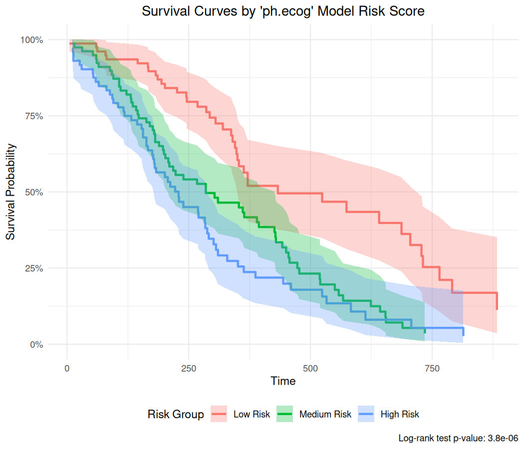
Show tidy table result as pretty table:
br_show_table(mds)
#>    Focal_variable      term estimate std.error statistic p.value     conf.int
#> 1         ph.ecog  ph.ecog1     1.51      0.20      2.05  0.040  [1.02, 2.23]
#> 2         ph.ecog  ph.ecog2     2.47      0.23      3.96  < .001 [1.58, 3.86]
#> 3         ph.ecog       age     1.01  9.31e-03      1.16  0.247  [0.99, 1.03]
#> 4         ph.ecog       sex     0.58      0.17     -3.24  0.001  [0.42, 0.81]
#> 5        ph.karno  ph.karno     0.99  5.95e-03     -2.06  0.040  [0.98, 1.00]
#> 6        ph.karno       age     1.01  9.46e-03      1.33  0.182  [0.99, 1.03]
#> 7        ph.karno       sex     0.62      0.17     -2.88  0.004  [0.44, 0.86]
#> 8       pat.karno pat.karno     0.98  5.68e-03     -3.30  < .001 [0.97, 0.99]
#> 9       pat.karno       age     1.01  9.38e-03      1.24  0.213  [0.99, 1.03]
#> 10      pat.karno       sex     0.60      0.17     -2.98  0.003  [0.43, 0.84]
#> 11       meal.cal  meal.cal     1.00  2.41e-04     -0.64  0.524  [1.00, 1.00]
#> 12       meal.cal       age     1.02      0.01      1.41  0.159  [0.99, 1.04]
#> 13       meal.cal       sex     0.62      0.19     -2.49  0.013  [0.43, 0.90]
#> 14        wt.loss   wt.loss     1.00  6.29e-03     -0.04  0.966  [0.99, 1.01]
#> 15        wt.loss       age     1.02  9.72e-03      2.05  0.040  [1.00, 1.04]
#> 16        wt.loss       sex     0.60      0.17     -2.90  0.004  [0.43, 0.85]
As markdown table:
br_show_table(mds, export = TRUE)
#> Focal_variable |      term | estimate | std.error | statistic | p.value |     conf.int
#> --------------------------------------------------------------------------------------
#> ph.ecog        |  ph.ecog1 |     1.51 |      0.20 |      2.05 |  0.040  | [1.02, 2.23]
#> ph.ecog        |  ph.ecog2 |     2.47 |      0.23 |      3.96 |  < .001 | [1.58, 3.86]
#> ph.ecog        |       age |     1.01 |  9.31e-03 |      1.16 |  0.247  | [0.99, 1.03]
#> ph.ecog        |       sex |     0.58 |      0.17 |     -3.24 |  0.001  | [0.42, 0.81]
#> ph.karno       |  ph.karno |     0.99 |  5.95e-03 |     -2.06 |  0.040  | [0.98, 1.00]
#> ph.karno       |       age |     1.01 |  9.46e-03 |      1.33 |  0.182  | [0.99, 1.03]
#> ph.karno       |       sex |     0.62 |      0.17 |     -2.88 |  0.004  | [0.44, 0.86]
#> pat.karno      | pat.karno |     0.98 |  5.68e-03 |     -3.30 |  < .001 | [0.97, 0.99]
#> pat.karno      |       age |     1.01 |  9.38e-03 |      1.24 |  0.213  | [0.99, 1.03]
#> pat.karno      |       sex |     0.60 |      0.17 |     -2.98 |  0.003  | [0.43, 0.84]
#> meal.cal       |  meal.cal |     1.00 |  2.41e-04 |     -0.64 |  0.524  | [1.00, 1.00]
#> meal.cal       |       age |     1.02 |      0.01 |      1.41 |  0.159  | [0.99, 1.04]
#> meal.cal       |       sex |     0.62 |      0.19 |     -2.49 |  0.013  | [0.43, 0.90]
#> wt.loss        |   wt.loss |     1.00 |  6.29e-03 |     -0.04 |  0.966  | [0.99, 1.01]
#> wt.loss        |       age |     1.02 |  9.72e-03 |      2.05 |  0.040  | [1.00, 1.04]
#> wt.loss        |       sex |     0.60 |      0.17 |     -2.90 |  0.004  | [0.43, 0.85]
As HTML table:
br_show_table(mds, export = TRUE, args_table_export = list(format = "html"))All functions are documented in the package reference, with full documentation available on the package site.
covr::package_coverage()If you use bregr in academic field, please cite:
(GPL-3) Copyright (c) 2025 Shixiang Wang & WangLabCSU team
These binaries (installable software) and packages are in development.
They may not be fully stable and should be used with caution. We make no claims about them.
Health stats visible at Monitor.