The hardware and bandwidth for this mirror is donated by dogado GmbH, the Webhosting and Full Service-Cloud Provider. Check out our Wordpress Tutorial.
If you wish to report a bug, or if you are interested in having us mirror your free-software or open-source project, please feel free to contact us at mirror[@]dogado.de.
2021-08-19
install.packages("bootf2", repos = "https://cloud.r-project.org/")# Need devtools. if you don't have it, install.packages("devtools")
devtools::install_github("zhengguoxu/bootf2")The package bootf2 was developed to compare the
dissolution profiles using bootstrap f2 method, as
recommended recently by several regulatory guidelines1–4. Several additional functions
were included later for the simulation of the dissolution profiles.
Currently, there are four main functions in the package:
sim.dp() to simulate dissolution profiles using
mathematical models or multivariate normal distribution. See vignette
Simulation of Dissolution Profiles on CRAN for
details.calcf2() to calculate similarity factor
f2 according to different regulatory rules. See
vignette Calculating Similarity Factor f2
on CRAN for
details.sim.dp.byf2() to find a dissolution profile that, when
compared to a given reference profile, has f2 value
equal to the predefined target f2. See vignette
Simulation of Dissolution Profiles with Predefined Target
f2 on CRAN for
details.bootf2() to estimate the confidence intervals of
f2s using bootstrap method. See vignette
Confidence Intervals of f2 Using Bootstrap Method on CRAN for
details.In addition to the vignettes for the main functions, some common topics such as regulation rules are discussed in the vignette Introduction to bootf2 on CRAN.
The most basic usage is given below as a brief demonstration.
sim.dp()The complete list of arguments are shown below. Read the function
manual with ?sim.dp for more details.
dat <- sim.dp(tp, dp, dp.cv, model = c("Weibull", "first-order"),
              model.par = NULL, seed = NULL, n.units = 12L, product,
              max.disso = 100, ascending = FALSE, message = FALSE,
              time.unit = c("min", "h"), plot = TRUE,
              plot.max.unit = 36L)
For the most basic use, the function can be run without any user
provided arguments, e.g., sim.dp(). In such case, 12 units
of individual dissolution profiles will be simulated using Weibull model
with a typical sampling time points of 5, 10, 15, 20, 30, 45, and 60
min. A seed number will be randomly generated, if not
provided by the user, and included in the output for reproducibility
purpose.
library(bootf2)
# simulation. simple as that.
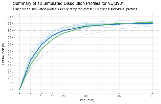
d.ref <- sim.dp(seed = 1234)
The output of sim.dp() is a list of at least 3
components:
sim.summary: A data frame with summary
statistics of all individual dissolution profiles.print(d.ref$sim.summary)
# product time dp dp.cv sim.mean sim.median sim.cv sim.var sim.sd
# 1 VCI3901 0 0.00000 NA 0.00000 0.00000 0.000000 0.000000 0.000000
# 2 VCI3901 5 35.91205 NA 42.59002 41.74175 19.312496 67.653855 8.225196
# 3 VCI3901 10 58.37878 NA 65.24386 64.63399 11.048803 51.964863 7.208666
# 4 VCI3901 15 72.55031 NA 77.95186 79.42119 8.856818 47.665970 6.904055
# 5 VCI3901 20 81.51082 NA 85.00156 86.16105 7.383728 39.391744 6.276284
# 6 VCI3901 30 90.78021 NA 91.34221 92.78433 4.956413 20.496418 4.527297
# 7 VCI3901 45 95.42728 NA 94.32405 95.06778 3.258574 9.447131 3.073618
# 8 VCI3901 60 96.61781 NA 95.21829 95.38719 2.752588 6.869471 2.620968
# sim.min sim.max sim.qt05 sim.qt25 sim.qt75 sim.qt95
# 1 0.00000 0.00000 0.00000 0.00000 0.00000 0.00000
# 2 28.86682 56.23244 30.08120 38.28761 48.65758 53.69296
# 3 48.29650 76.37401 54.49829 62.94728 69.54749 74.58668
# 4 60.03121 85.53969 66.92377 75.59784 82.76237 84.65364
# 5 68.43588 92.13902 75.32032 82.27256 88.85582 90.96216
# 6 79.25227 96.60286 84.06618 89.90644 93.51285 95.88751
# 7 87.54060 99.40223 88.90028 93.78673 95.48357 98.00911
# 8 90.36151 99.80318 90.94327 94.12407 96.65417 98.79344sim.disso: A data frame with all individual
dissolution profiles.print(d.ref$sim.disso)
# time unit.01 unit.02 unit.03 unit.04 unit.05 unit.06 unit.07 unit.08
# 1 0 0.00000 0.00000 0.00000 0.00000 0.00000 0.00000 0.00000 0.00000
# 2 5 42.44302 38.68705 47.76202 31.07478 28.86682 41.04047 40.98547 51.34429
# 3 10 64.34095 59.57248 68.16946 48.29650 63.68414 64.92703 61.81370 73.12431
# 4 15 76.12156 72.56313 79.54749 60.03121 83.92869 78.42522 74.02670 83.83484
# 5 20 82.53928 80.95304 86.33855 68.43588 92.13902 85.98356 81.47238 89.33110
# 6 30 88.00484 90.19166 93.22817 79.25227 95.30223 92.52769 89.05079 93.77081
# 7 45 90.01275 95.58009 96.86928 87.54060 95.45140 94.92385 92.93529 95.32524
# 8 60 90.36151 97.34724 97.96729 91.41926 95.45178 95.32260 94.01854 95.59138
# unit.09 unit.10 unit.11 unit.12
# 1 0.00000 0.00000 0.00000 0.00000
# 2 43.93941 56.23244 51.61520 37.08931
# 3 69.44566 76.37401 69.85299 63.32513
# 4 82.40489 85.53969 79.70409 79.29489
# 5 88.69740 89.99927 85.58302 88.54620
# 6 93.04097 93.42686 91.70737 96.60286
# 7 94.07055 94.56556 95.21171 99.40223
# 8 94.15925 94.75433 96.42314 99.80318sim.info: A data frame with information of the
simulation.print(d.ref$sim.info)
# fmax fmax.cv mdt mdt.cv beta beta.cv tlag tlag.cv seed n.units
# 1 97.03 3 10.87 30 0.993764 20 0 0 1234 12
# max.disso model time.unit
# 1 100 Weibull minDepending on the argument settings, there might be two additional components:
model.par.ind: A data frame of individual
model parameters that are used to simulate the individual dissolution
profiles if mathematical models are chosen for the simulation.print(d.ref$model.par.ind)
# fmax.ind mdt.ind beta.ind tlag.ind
# 1 90.43662 7.995749 0.9720844 0
# 2 98.28721 10.820746 0.8972171 0
# 3 98.51432 8.208926 0.8282050 0
# 4 95.37133 15.130249 0.8405575 0
# 5 95.45179 9.424652 1.6110909 0
# 6 95.40077 8.786133 1.0207750 0
# 7 94.47347 9.352365 0.9008715 0
# 8 95.65084 6.667725 0.9099505 0
# 9 94.16689 7.657771 1.0894384 0
# 10 94.79651 5.651917 0.8650227 0
# 11 97.21781 7.269654 0.7438644 0
# 12 99.86358 9.951453 1.1148230 0sim.plot: A plot if plot = TRUE.print(d.ref$sim.plot)
Simple case like this might be useful in situations such as testing
other programs where data with certain format is needed. In general, to
have better controlled outcomes, argument tp,
model, and model.par should be provided.
calcf2()The complete list of arguments are shown below. Read the function
manual with ?calcf2 for more details. In addition, refer to
the vignette Introduction to bootf2 on CRAN for detailed
discussion on different regulatory requirements regarding to the
applicability of f2.
calcf2(test, ref, path.in, file.in, path.out, file.out,
       regulation = c("EMA", "FDA", "WHO", "Canada", "ANVISA"),
       cv.rule = TRUE, message = FALSE, min.points = 3L,
       f2.type = c("est.f2", "exp.f2", "bc.f2", "vc.exp.f2",
                   "vc.bc.f2", "all"), both.TR.85 = FALSE,
       digits = 2L, time.unit = c("min", "h"),  plot = TRUE,
       plot.start.time = 0, plot.max.unit = 24L)
The minimum required arguments are test and
ref. Data can also be read from an Excel file. For
interactive use, such as the examples below, the test and
ref should be data frames with the time as the first
column and individual profiles as the rest columns. The
sim.disso data frame in the output of sim.dp()
comes with the correct format, as shown above. This is the base function
used by function bootf2().
# simulate a test data
d.test <- sim.dp(seed = 100, plot = FALSE, message = TRUE)
# Dissolution data was generated using Weibull model, with the
# following model parameters:
# - fmax      = 98.75
# - fmax.cv   = 3%
# - tlag      = 0
# - tlag.cv   = 0%
# - mdt       = 10.4
# - mdt.cv    = 30%
# - beta      = 0.787472
# - beta.cv   = 20%
#
# Seed number used:  100

# calculate f2 with default settings
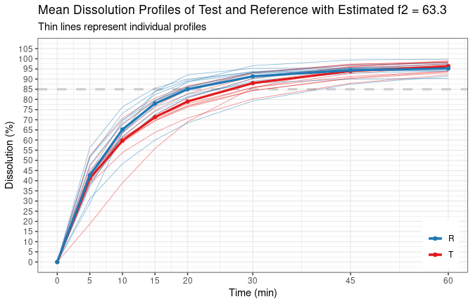
tmp.f2 <- calcf2(d.test$sim.disso, d.ref$sim.disso, message = TRUE)
# The f2 method was applied according to EMA's BE guideline.
#
# Individual data was provided with option 'cv.rule = TRUE',
# therefore, CV has been calculated and checked accordingly.
#
# Calculated mean and CV as follows:
# Time   Mean (T)   Mean (R)     CV (T)     CV (R)
# 5         41.09      42.59      19.64      19.31
# 10        59.69      65.24      13.12      11.05
# 15        71.29      77.95       9.39       8.86
# 20        79.00      85.00       7.10       7.38
# ------------------------------------------------
# 30        88.00      91.34       4.82       4.96
# 45        93.95      94.32       3.41       3.26
# 60        96.35      95.22       2.55       2.75
# ==================================
# Number of units for test is      : nt = 12
# Number of units for reference is : nr = 12
#
# CV criteria fulfilled; therefore, f2 method can be applied.
#
# The time points above the dashed line are used in f2 calculation.
#
# Estimated f2 = 63.3
print(tmp.f2)
#   f2.type f2.value f2.tp d85at15 regulation cv.rule min.points
# 1  est.f2 63.29838     4      no        EMA    TRUE          3
When the conditions to apply f2 are not fulfilled, the function will stop and, depending on the details of non-compliance of regulatory rules, show different error messages.
# simulate reference profile with CV% criterion not fulfilled
d.ref2 <- sim.dp(seed = 456)

# output with error message
calcf2(d.test$sim.disso, d.ref2$sim.disso, message = TRUE)
# The f2 method was applied according to EMA's BE guideline.
#
# Individual data was provided with option 'cv.rule = TRUE',
# therefore, CV has been calculated and checked accordingly.
#
# Calculated mean and CV as follows:
# Time   Mean (T)   Mean (R)     CV (T)     CV (R)
# 5         41.09      34.09      19.64      30.50
# 10        59.69      56.34      13.12      20.10
# 15        71.29      70.71       9.39      16.24
# 20        79.00      79.66       7.10      13.48
# 30        88.00      88.70       4.82       9.01
# ------------------------------------------------
# 45        93.95      93.58       3.41       5.27
# 60        96.35      95.33       2.55       3.75
# ==================================
# Number of units for test is      : nt = 12
# Number of units for reference is : nr = 12
#
# CV criteria not fulfilled; therefore, f2 method cannot be applied.
# Error in calcf2(d.test$sim.disso, d.ref2$sim.disso, message = TRUE): You should consider alternative methods such as bootstrap f2.sim.dp.byf2()The complete list of arguments are shown below. Read the function
manual with ?sim.dp.byf2 for more details.
dat <- sim.dp.byf2(tp, dp, target.f2, seed = NULL, min.points = 3L,
                   regulation = c("EMA", "FDA", "WHO", "Canada", "ANVISA"),
                   model = c("Weibull", "first-order"), digits = 2L,
                   max.disso = 100, message = FALSE, both.TR.85 = FALSE,
                   time.unit = c("min", "h"), plot = TRUE, sim.dp.out,
                   sim.target = c("ref.pop", "ref.median", "ref.mean"),
                   model.par.cv = 50, fix.fmax.cv = 0, random.factor = 3)
Given any dissolution profile dp at time points
tp, and target f2 value (e.g.,
target.f2 = 55), this function will find another
dissolution profile such that when the newly simulated profile is
compared to the dp, the calculated f2
will be equal to the target f2. If
target.f2 is provided as a range, such as
target.f2 = c(54.95, 55.04), then the calculated
f2 with simulated profile will be within this
range.
# mean dissolution profile for tp
tp <- c(5, 10, 15, 20, 30, 45, 60)
dp <- c(51, 66, 75, 81, 88, 92, 95)

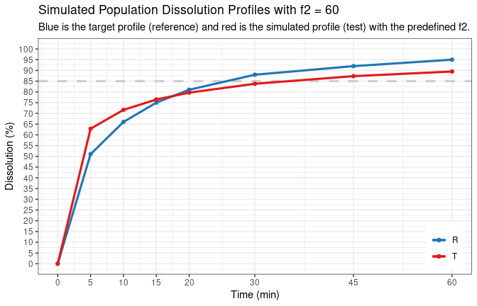
# find another profile with target f2 = 60
d.t2 <- sim.dp.byf2(tp, dp, target.f2 = 60, seed = 123, message = TRUE)
# Obtained model parameters and calculated f2 are:
#     model seed     fmax tlag      mdt      beta f2 f2.tp regulation
# 1 Weibull  123 96.95502    0 4.424869 0.3611346 60     5        EMA
#
# And the difference between simulated test and reference is:
#   time ref     test   diff.tr
# 1    0   0  0.00000  0.000000
# 2    5  51 62.86075 11.860752
# 3   10  66 71.62829  5.628286
# 4   15  75 76.46007  1.460075
# 5   20  81 79.66658 -1.333418
# 6   30  88 83.78233 -4.217670
# 7   45  92 87.33950 -4.660501
# 8   60  95 89.48884 -5.511159
The model parameters in the output are more useful in simulation
studies since they can be used as initial model parameter input to the
function sim.dp() to simulate a large population of
individual dissolution profiles that have the known population
f2 value when compared to target dissolution
profile.
bootf2()The complete list of arguments are shown below. Read the function
manual with ?bootf2 for more details.
result <- bootf2(test, ref, path.in, file.in, path.out, file.out,
                 n.boots = 10000L, seed = 306L, digits = 2L, alpha = 0.05,
                 regulation = c("EMA", "FDA", "WHO", "Canada", "ANVISA"),
                 min.points = 1L, both.TR.85 = FALSE, print.report = TRUE,
                 report.style = c("concise",  "intermediate", "detailed"),
                 f2.type = c("all", "est.f2", "exp.f2", "bc.f2",
                             "vc.exp.f2", "vc.bc.f2"),
                 ci.type = c("all", "normal", "basic", "percentile",
                             "bca.jackknife", "bca.boot"),
                 quantile.type = c("all", as.character(1:9), "boot"),
                 jackknife.type = c("all", "nt+nr", "nt*nr", "nt=nr"),
                 time.unit = c("min", "h"), output.to.screen = FALSE,
                 sim.data.out = FALSE)
The minimum required arguments are dissolution profiles of
test and ref. The function can output many
different 90% confidence intervals for several f2
estimators. With default settings, the function prints all confidence
intervals for all f2 estimators, and the result will
be save in a text file.
# get test and reference data set with correct format
test <- d.test$sim.disso
ref  <- d.ref$sim.disso

# use most default settings (output all) but small number of bootstrap
# to have shorter run time for the example. default n.boots = 10000L
t_vs_r <- bootf2(test, ref, n.boots = 100L, print.report = FALSE,
                 output.to.screen = TRUE)
# =================================================================
# |                                                               |
# |  Comparison of Dissolution Profiles by Bootstrap f2 Method.   |
# |_______________________________________________________________|
# |                                                               |
# | Smimilarity Criterion:                                        |
# | ----------------------                                        |
# |     To conclude similarity, the lower limit of 90% confidence |
# | interval should be greater than or equal to 50.               |
# |                                                               |
# =================================================================
#
# =================================================================
# * T & R dissolved more than 85% at 15 min in original data : NO |
# =================================================================
#
# ============================================
# |              Main Results:               |
# |  f2 and Its Confidence Intervals (CI)s   |
# ============================================
#
# -------------------------------
# * Estimated f2 Values (est.f2)
# -------------------------------
#   - with original data                        :   63.3
#   - with original data (by Jackknife, nt+nr)  :   63.8
#   - with original data (by Jackknife, nt*nr)  :   64.29
#   - with original data (by Jackknife, nt=nr)  :   64.37
#   - with bootstrapped data (Mean)             :   65.22
#   - with bootstrapped data (Median)           :   64.13
#
# -----------------------
# * Confidence Intervals
# -----------------------
#           Types of         Lower   Upper
#     Confidence Intervals   <----------->
#                   Normal   45.80   76.95
#                    Basic   44.15   73.55
#      Percentile (Type 1)   53.02   82.24
#      Percentile (Type 2)   53.28   82.35
#      Percentile (Type 3)   53.02   82.24
#      Percentile (Type 4)   53.02   82.24
#      Percentile (Type 5)   53.28   82.35
#      Percentile (Type 6)   53.05   82.44
#      Percentile (Type 7)   53.50   82.25
#      Percentile (Type 8)   53.20   82.38
#      Percentile (Type 9)   53.22   82.37
#        Percentile (boot)   53.05   82.44
#   BCa (jackknife, nt+nr)   47.56   81.00
#   BCa (jackknife, nt*nr)   47.35   80.91
#   BCa (jackknife, nt=nr)   47.08   80.80
#               BCa (boot)   49.37   81.73
# ------------------------------------------------------------
#   Out of 100 bootstrapped data sets,
#   - Number of f2 calculated with 1 time point             :   0
#   - Number of f2 calculated with 2 time point             :   0
#   - Number of f2 cannot be calculated (NA)                :   0
#   - Number of T and R dissolving more than 85% at 15 min  :   0
# ------------------------------------------------------------
# ______________________________________________________________________
#
# ------------------------------
# * Expected f2 Values (exp.f2)
# ------------------------------
#   - with original data                        :   60.53
#   - with original data (by Jackknife, nt+nr)  :   60.89
#   - with original data (by Jackknife, nt*nr)  :   61.24
#   - with original data (by Jackknife, nt=nr)  :   61.3
#   - with bootstrapped data (Mean)             :   61.73
#   - with bootstrapped data (Median)           :   62.05
#
# -----------------------
# * Confidence Intervals
# -----------------------
#           Types of         Lower   Upper
#     Confidence Intervals   <----------->
#                   Normal   48.25   70.41
#                    Basic   48.74   69.65
#      Percentile (Type 1)   51.40   71.78
#      Percentile (Type 2)   51.56   72.06
#      Percentile (Type 3)   51.40   71.78
#      Percentile (Type 4)   51.40   71.78
#      Percentile (Type 5)   51.56   72.06
#      Percentile (Type 6)   51.41   72.32
#      Percentile (Type 7)   51.71   71.81
#      Percentile (Type 8)   51.51   72.15
#      Percentile (Type 9)   51.53   72.13
#        Percentile (boot)   51.42   72.32
#   BCa (jackknife, nt+nr)   45.03   70.53
#   BCa (jackknife, nt*nr)   45.10   70.55
#   BCa (jackknife, nt=nr)   44.98   70.51
#               BCa (boot)   45.03   70.53
# ------------------------------------------------------------
#   Out of 100 bootstrapped data sets,
#   - Number of f2 calculated with 1 time point             :   0
#   - Number of f2 calculated with 2 time point             :   0
#   - Number of f2 cannot be calculated (NA)                :   0
#   - Number of T and R dissolving more than 85% at 15 min  :   0
# ------------------------------------------------------------
# ______________________________________________________________________
#
# -----------------------------------
# * Bias-Corrected f2 Values (bc.f2)
# -----------------------------------
#   - with original data                        :   67.02
#   - with original data (by Jackknife, nt+nr)  :   67.82
#   - with original data (by Jackknife, nt*nr)  :   68.65
#   - with original data (by Jackknife, nt=nr)  :   68.78
#   - with bootstrapped data (Mean)             :   67.95
#   - with bootstrapped data (Median)           :   65.61
#
# -----------------------
# * Confidence Intervals
# -----------------------
#           Types of         Lower   Upper
#     Confidence Intervals   <----------->
#                   Normal   47.10   85.09
#                    Basic   42.05   80.87
#      Percentile (Type 1)   54.53   91.49
#      Percentile (Type 2)   54.53   91.49
#      Percentile (Type 3)   54.53   89.91
#      Percentile (Type 4)   52.89   90.54
#      Percentile (Type 5)   54.54   91.33
#      Percentile (Type 6)   53.09   92.02
#      Percentile (Type 7)   54.57   90.62
#      Percentile (Type 8)   54.32   91.57
#      Percentile (Type 9)   54.48   91.51
#        Percentile (boot)   53.17   91.99
#   BCa (jackknife, nt+nr)   54.53   92.61
#   BCa (jackknife, nt*nr)   53.49   92.11
#   BCa (jackknife, nt=nr)   53.88   92.26
#               BCa (boot)   54.60   93.66
# ------------------------------------------------------------
#   Out of 100 bootstrapped data sets,
#   - Number of f2 calculated with 1 time point             :   0
#   - Number of f2 calculated with 2 time point             :   0
#   - Number of f2 cannot be calculated (NA)                :   8
#   - Number of T and R dissolving more than 85% at 15 min  :   0
# ------------------------------------------------------------
# ______________________________________________________________________
#
# ----------------------------------------------------
# * Variance-corrected Expected f2 Values (vc.exp.f2)
# ----------------------------------------------------
#   - with original data                        :   60.53
#   - with original data (by Jackknife, nt+nr)  :   60.87
#   - with original data (by Jackknife, nt*nr)  :   61.21
#   - with original data (by Jackknife, nt=nr)  :   61.26
#   - with bootstrapped data (Mean)             :   61.54
#   - with bootstrapped data (Median)           :   61.98
#
# -----------------------
# * Confidence Intervals
# -----------------------
#           Types of         Lower   Upper
#     Confidence Intervals   <----------->
#                   Normal   48.60   70.43
#                    Basic   49.07   69.66
#      Percentile (Type 1)   51.37   70.98
#      Percentile (Type 2)   51.49   71.51
#      Percentile (Type 3)   51.37   70.98
#      Percentile (Type 4)   51.37   70.98
#      Percentile (Type 5)   51.49   71.51
#      Percentile (Type 6)   51.39   71.99
#      Percentile (Type 7)   51.60   71.03
#      Percentile (Type 8)   51.46   71.67
#      Percentile (Type 9)   51.47   71.63
#        Percentile (boot)   51.39   71.98
#   BCa (jackknife, nt+nr)   44.93   70.12
#   BCa (jackknife, nt*nr)   44.99   70.14
#   BCa (jackknife, nt=nr)   44.88   70.08
#               BCa (boot)   44.88   70.09
# ------------------------------------------------------------
#   Out of 100 bootstrapped data sets,
#   - Number of f2 calculated with 1 time point             :   0
#   - Number of f2 calculated with 2 time point             :   0
#   - Number of f2 cannot be calculated (NA)                :   0
#   - Number of T and R dissolving more than 85% at 15 min  :   0
# ------------------------------------------------------------
# ______________________________________________________________________
#
# ----------------------------------------------------
# * Variance- and Bias-Corrected f2 Values (vc.bc.f2)
# ----------------------------------------------------
#   - with original data                        :   67.03
#   - with original data (by Jackknife, nt+nr)  :   67.87
#   - with original data (by Jackknife, nt*nr)  :   68.74
#   - with original data (by Jackknife, nt=nr)  :   68.86
#   - with bootstrapped data (Mean)             :   68.48
#   - with bootstrapped data (Median)           :   66.01
#
# -----------------------
# * Confidence Intervals
# -----------------------
#           Types of         Lower   Upper
#     Confidence Intervals   <----------->
#                   Normal   45.50   85.65
#                    Basic   39.60   80.75
#      Percentile (Type 1)   54.69   94.30
#      Percentile (Type 2)   54.69   94.30
#      Percentile (Type 3)   54.69   90.50
#      Percentile (Type 4)   53.02   92.02
#      Percentile (Type 5)   54.69   93.92
#      Percentile (Type 6)   53.23   94.47
#      Percentile (Type 7)   54.72   92.21
#      Percentile (Type 8)   54.48   94.32
#      Percentile (Type 9)   54.63   94.30
#        Percentile (boot)   53.31   94.46
#   BCa (jackknife, nt+nr)   54.65   94.62
#   BCa (jackknife, nt*nr)   53.49   94.48
#   BCa (jackknife, nt=nr)   53.59   94.49
#               BCa (boot)   54.76   97.00
# ------------------------------------------------------------
#   Out of 100 bootstrapped data sets,
#   - Number of f2 calculated with 1 time point             :   0
#   - Number of f2 calculated with 2 time point             :   0
#   - Number of f2 cannot be calculated (NA)                :   8
#   - Number of T and R dissolving more than 85% at 15 min  :   0
# ------------------------------------------------------------
# ______________________________________________________________________
#
# ============================================
# | Function Settings and System Information |
# ============================================
#
# ---------------------
# * Function Settings
# ---------------------
#   - test              :   test
#   - ref               :   ref
#   - n.boots           :   100
#   - seed              :   306
#   - digits            :   2
#   - alpha             :   0.05 (90% CI)
#   - regulation        :   EMA
#   - min.points        :   1
#   - both.TR.85        :   FALSE
#   - print.report      :   FALSE
#   - report.style      :   concise (not used)
#   - f2.type           :   all
#   - ci.type           :   all
#   - quantile.type     :   all
#   - jackknife.type    :   all
#   - time.unit         :   min
#   - output.to.screen  :   TRUE
#   - sim.data.out      :   FALSE
#   - path.in           :   Not provided
#   - file.in           :   Not provided
#   - path.out          :   Not provided
#   - file.out          :   Not provided
#
# ---------------------
# * System Information
# ---------------------
#   - OS Platform             :   x86_64-pc-linux-gnu (64-bit)
#   - OS Name and Release     :   Ubuntu 20.04.2 LTS
#   - Machine Node Name       :   MyHomeLinuxPC
#   - User Name               :   zhengguo
#   - Time Zone               :   Europe/Madrid
#   - R Version               :   4.1.1 (2021-08-10)
#   - Package bootf2 Version  :   0.4.0.9000
# ______________________________________________________________________
The output of the bootf2() is a list
containing: 1. boot.ci: A data frame of bootstrap
f2 confidence intervals. 1. boot.f2: A
data frame of all individual f2 values for
all bootstrap data sets. This can be used to make plots for visual
presentation. 1. boot.info: A data frame with
detailed information of bootstrap for reproducibility purpose, such as
all arguments used in the function, time points used for calculation of
, and the number of NAs. 1. boot.summary: A
data frame with descriptive statistics of the bootstrap
f2.
And depending on the function settings, it might contains
boot.t and boot.r, lists of all individual
bootstrap data sets for the test and reference products.
Despite the best efforts the author has put into, the package is offered without any guarantee of accuracy and absolutely no warranty. Validation of the package, especially when it is used in regulatory field, is the responsibility of the users. The author accept absolutely no liability for any financial loss or risk to public health resulting from the use of this package.
These binaries (installable software) and packages are in development.
They may not be fully stable and should be used with caution. We make no claims about them.
Health stats visible at Monitor.