README

The hardware and bandwidth for this mirror is donated by dogado GmbH, the Webhosting and Full Service-Cloud Provider. Check out our Wordpress Tutorial.
If you wish to report a bug, or if you are interested in having us mirror your free-software or open-source project, please feel free to contact us at mirror[@]dogado.de.

blueterra

blueterra is an R package for geomorphometric analysis of submerged terrain. It works from user-supplied bathymetric or elevation rasters and provides workflows for deriving terrain metrics, organizing metrics into process-oriented groups, and summarizing seafloor structure across polygons, transects, depth bands, and isobath corridors.

For a complete worked example using the installed example rasters, see the Get Started article.

Installation

install.packages("remotes")
remotes::install_github("el-cordero/blueterra")

install.packages("path/to/blueterra", repos = NULL, type = "source")

Example Data

The installed examples are reduced from analysis rasters and sampling rectangles used to test terrain workflows on real shelf-margin morphology. They are compact enough for package examples, but they retain depth gradients, slope breaks, local relief, and sampling-rectangle geometry.

library(blueterra)
library(terra)

hitw <- read_bathy(blueterra_example("hitw"))
hoyo <- read_bathy(blueterra_example("hoyo"))
slope <- read_bathy(blueterra_example("slope"))
rectangles <- terra::vect(blueterra_example("sampling_rectangles"))

hitw_rect <- rectangles[rectangles$site_id == "hitw", ]

examples <- blueterra_examples()
examples$path <- basename(examples$path)
examples
#> # A tibble: 6 × 8
#>   name                path     type  description crs    nrow  ncol feature_count
#>   <chr>               <chr>    <chr> <chr>       <chr> <dbl> <dbl>         <dbl>
#> 1 hitw                lapargu… rast… Reduced Ho… +pro…    75    75            NA
#> 2 hoyo                lapargu… rast… Reduced El… +pro…   123   124            NA
#> 3 slope               lapargu… rast… Aggregated… +pro…    90   190            NA
#> 4 sampling_rectangles lapargu… vect… Sampling r… +pro…    NA    NA             3
#> 5 synthetic_bathy     synthet… rast… Synthetic … +pro…    60    60            NA
#> 6 synthetic_zones     synthet… vect… Synthetic … +pro…    NA    NA             2

Quick Start

This compact workflow reads Hole-in-the-Wall bathymetry, checks the raster assumptions, prepares the surface, derives a focused terrain stack, and summarizes metrics inside the sampling rectangle.

bathy_info(hitw)
#> # A tibble: 1 × 13
#>   layer    nrow  ncol ncell    xmin   xmax   ymin   ymax  xres  yres   min   max
#>   <chr>   <dbl> <dbl> <dbl>   <dbl>  <dbl>  <dbl>  <dbl> <dbl> <dbl> <dbl> <dbl>
#> 1 bathy_m    75    75  5625 137474. 1.38e5 2.06e5 2.06e5  4.00  4.00 -269. -16.6
#> # ℹ 1 more variable: crs <chr>

hitw_prepared <- prepare_bathy(
  hitw,
  depth_range = c(-220, -25),
  smooth = TRUE,
  smooth_window = 3
)

hitw_metrics <- derive_terrain(
  hitw_prepared,
  metrics = c("slope", "aspect", "northness", "eastness", "tri", "rugosity",
              "bpi", "curvature", "surface_area_ratio")
)

terrain_summary <- summarize_terrain(
  hitw_metrics,
  hitw_rect,
  fun = c("mean", "sd", "min", "max")
)

names(hitw_metrics)
#>  [1] "slope_deg"          "aspect_deg"         "northness"         
#>  [4] "eastness"           "tri"                "rugosity_vrm_3x3"  
#>  [7] "bpi_3x3"            "bpi_11x11"          "curvature"         
#> [10] "surface_area_ratio"
terrain_summary[, c("site_id", "site_name", "slope_deg_mean", "bpi_3x3_mean")]
#> # A tibble: 1 × 4
#>   site_id site_name        slope_deg_mean bpi_3x3_mean
#>   <chr>   <chr>                     <dbl>        <dbl>
#> 1 hitw    Hole-in-the-Wall           50.9      0.00568

Depth sign conventions are preserved unless conversion is requested explicitly. The example rasters are stored as negative elevation, so larger numeric values are shallower and smaller values are deeper.

Key Figures

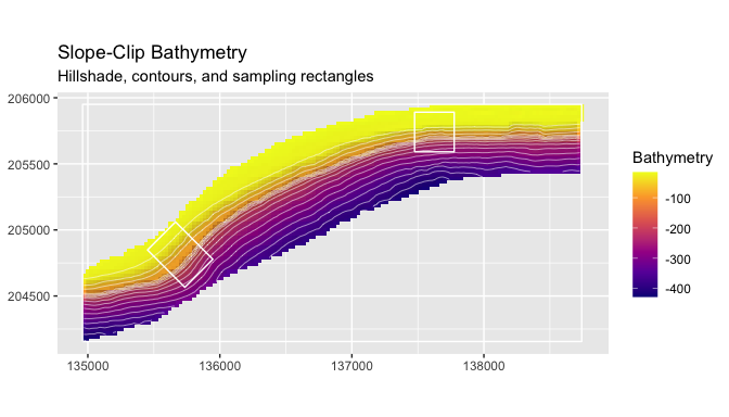
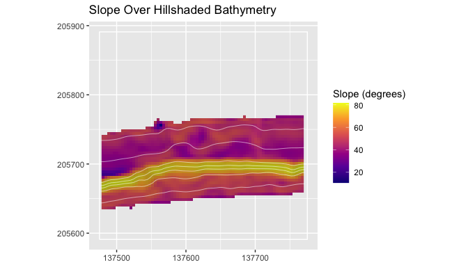
Hillshade is used in these figures as visual relief. It helps the reader see the terrain form behind contours, vectors, and metric layers; it is not a model predictor unless the analyst chooses to include it.

plot_bathy(
  slope,
  contours = TRUE,
  contour_interval = 25,
  vectors = rectangles,
  title = "Slope-Clip Bathymetry",
  subtitle = "Hillshade, contours, and sampling rectangles"
)

plot_metric(
  hitw_metrics,
  metric = "slope_deg",
  bathy = hitw_prepared,
  contours = TRUE,
  contour_interval = 25,
  vectors = hitw_rect,
  title = "Slope Over Hillshaded Bathymetry",
  legend_title = "Slope (degrees)"
)

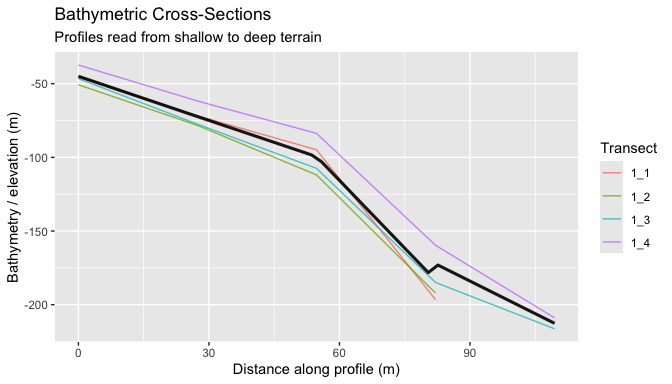
transects <- make_transects(hitw_rect, spacing = 75, bathy = hitw_prepared)
cross_sections <- sample_transects(transects, hitw_prepared, n = 12)

plot_cross_sections(
  cross_sections,
  value_col = "bathy_m",
  mean_profile = TRUE,
  mean_profile_na_rm = TRUE,
  normalize_distance = FALSE,
  profile_direction = "top_to_bottom",
  title = "Bathymetric Cross-Sections",
  subtitle = "Profiles read from shallow to deep terrain"
)

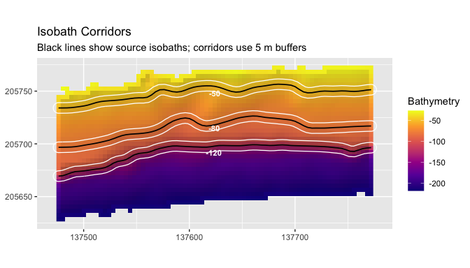
isobaths <- extract_isobaths(hitw_prepared, depths = c(-50, -80, -120))
corridors <- make_isobath_corridors(
  hitw_prepared,
  depths = c(-50, -80, -120),
  width = 5
)

plot_isobath_corridors(
  corridors,
  hitw_prepared,
  isobaths = isobaths,
  background_contours = FALSE,
  title = "Isobath Corridors",
  subtitle = "Black lines show source isobaths; corridors use 5 m buffers"
)

Articles

Citation

Please cite blueterra with the package citation once the release metadata are finalized:

citation("blueterra")

License

These binaries (installable software) and packages are in development.
They may not be fully stable and should be used with caution. We make no claims about them.
Health stats visible at Monitor.