The hardware and bandwidth for this mirror is donated by dogado GmbH, the Webhosting and Full Service-Cloud Provider. Check out our Wordpress Tutorial.
If you wish to report a bug, or if you are interested in having us mirror your free-software or open-source project, please feel free to contact us at mirror[@]dogado.de.
Tools for building binary logistic regression models
![]()
![]()
Tools designed to make it easier for users, particularly beginner/intermediate R users to build logistic regression models. Includes comprehensive regression output, variable selection procedures, model validation techniques and a ‘shiny’ app for interactive model building.
# Install blorr from CRAN
install.packages("blorr")

# Install development version from GitHub
# install.packages("devtools")
devtools::install_github("rsquaredacademy/blorr")

# Install the development version from `rsquaredacademy` universe
install.packages("blorr", repos = "https://rsquaredacademy.r-universe.dev")blorr uses consistent prefix blr_* for easy tab
completion.
library(blorr)
library(magrittr)blr_bivariate_analysis(hsb2, honcomp, female, prog, race, schtyp)
#> Bivariate Analysis
#> ---------------------------------------------------------------------
#> Variable Information Value LR Chi Square LR DF LR p-value
#> ---------------------------------------------------------------------
#> female 0.10 3.9350 1 0.0473
#> prog 0.43 16.1450 2 3e-04
#> race 0.33 11.3694 3 0.0099
#> schtyp 0.00 0.0445 1 0.8330
#> ---------------------------------------------------------------------blr_woe_iv(hsb2, prog, honcomp)
#> Weight of Evidence
#> -------------------------------------------------------------------------
#> levels count_0s count_1s dist_0s dist_1s woe iv
#> -------------------------------------------------------------------------
#> 1 38 7 0.26 0.13 0.67 0.08
#> 2 65 40 0.44 0.75 -0.53 0.17
#> 3 44 6 0.30 0.11 0.97 0.18
#> -------------------------------------------------------------------------
#>
#> Information Value
#> -----------------------------
#> Variable Information Value
#> -----------------------------
#> prog 0.4329
#> -----------------------------# create model using glm
model <- glm(honcomp ~ female + read + science, data = hsb2,
family = binomial(link = 'logit'))blr_regress(model)
#> Model Overview
#> ------------------------------------------------------------------------
#> Data Set Resp Var Obs. Df. Model Df. Residual Convergence
#> ------------------------------------------------------------------------
#> data honcomp 200 199 196 TRUE
#> ------------------------------------------------------------------------
#>
#> Response Summary
#> --------------------------------------------------------
#> Outcome Frequency Outcome Frequency
#> --------------------------------------------------------
#> 0 147 1 53
#> --------------------------------------------------------
#>
#> Maximum Likelihood Estimates
#> -----------------------------------------------------------------
#> Parameter DF Estimate Std. Error z value Pr(>|z|)
#> -----------------------------------------------------------------
#> (Intercept) 1 -12.7772 1.9755 -6.4677 0.0000
#> female1 1 1.4825 0.4474 3.3139 9e-04
#> read 1 0.1035 0.0258 4.0186 1e-04
#> science 1 0.0948 0.0305 3.1129 0.0019
#> -----------------------------------------------------------------
#>
#> Association of Predicted Probabilities and Observed Responses
#> ---------------------------------------------------------------
#> % Concordant 0.8561 Somers' D 0.7147
#> % Discordant 0.1425 Gamma 0.7136
#> % Tied 0.0014 Tau-a 0.2794
#> Pairs 7791 c 0.8568
#> ---------------------------------------------------------------blr_model_fit_stats(model)
#> Model Fit Statistics
#> ---------------------------------------------------------------------------------
#> Log-Lik Intercept Only: -115.644 Log-Lik Full Model: -80.118
#> Deviance(196): 160.236 LR(3): 71.052
#> Prob > LR: 0.000
#> MCFadden's R2 0.307 McFadden's Adj R2: 0.273
#> ML (Cox-Snell) R2: 0.299 Cragg-Uhler(Nagelkerke) R2: 0.436
#> McKelvey & Zavoina's R2: 0.518 Efron's R2: 0.330
#> Count R2: 0.810 Adj Count R2: 0.283
#> BIC: 181.430 AIC: 168.236
#> ---------------------------------------------------------------------------------blr_confusion_matrix(model)
#> Confusion Matrix and Statistics
#>
#> Reference
#> Prediction 0 1
#> 0 135 26
#> 1 12 27
#>
#>
#> Accuracy : 0.8100
#> No Information Rate : 0.7350
#>
#> Kappa : 0.4673
#>
#> McNemars's Test P-Value : 0.0350
#>
#> Sensitivity : 0.5094
#> Specificity : 0.9184
#> Pos Pred Value : 0.6923
#> Neg Pred Value : 0.8385
#> Prevalence : 0.2650
#> Detection Rate : 0.1350
#> Detection Prevalence : 0.1950
#> Balanced Accuracy : 0.7139
#> Precision : 0.6923
#> Recall : 0.5094
#>
#> 'Positive' Class : 1blr_test_hosmer_lemeshow(model)
#> Partition for the Hosmer & Lemeshow Test
#> --------------------------------------------------------------
#> def = 1 def = 0
#> Group Total Observed Expected Observed Expected
#> --------------------------------------------------------------
#> 1 20 0 0.16 20 19.84
#> 2 20 0 0.53 20 19.47
#> 3 20 2 0.99 18 19.01
#> 4 20 1 1.64 19 18.36
#> 5 21 3 2.72 18 18.28
#> 6 19 3 4.05 16 14.95
#> 7 20 7 6.50 13 13.50
#> 8 20 10 8.90 10 11.10
#> 9 20 13 11.49 7 8.51
#> 10 20 14 16.02 6 3.98
#> --------------------------------------------------------------
#>
#> Goodness of Fit Test
#> ------------------------------
#> Chi-Square DF Pr > ChiSq
#> ------------------------------
#> 4.4998 8 0.8095
#> ------------------------------blr_gains_table(model)
#> decile total 1 0 ks tp tn fp fn sensitivity specificity accuracy
#> 1 1 20 14 6 22.33346 14 141 6 39 26.41509 95.91837 77.5
#> 2 2 20 13 7 42.09986 27 134 13 26 50.94340 91.15646 80.5
#> 3 3 20 10 10 54.16506 37 124 23 16 69.81132 84.35374 80.5
#> 4 4 20 7 13 58.52907 44 111 36 9 83.01887 75.51020 77.5
#> 5 5 20 3 17 52.62482 47 94 53 6 88.67925 63.94558 70.5
#> 6 6 20 3 17 46.72058 50 77 70 3 94.33962 52.38095 63.5
#> 7 7 20 1 19 35.68220 51 58 89 2 96.22642 39.45578 54.5
#> 8 8 20 2 18 27.21088 53 40 107 0 100.00000 27.21088 46.5
#> 9 9 20 0 20 13.60544 53 20 127 0 100.00000 13.60544 36.5
#> 10 10 20 0 20 0.00000 53 0 147 0 100.00000 0.00000 26.5model %>%
blr_gains_table() %>%
plot()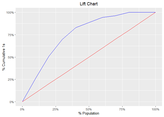
model %>%
  blr_gains_table() %>%
  blr_roc_curve()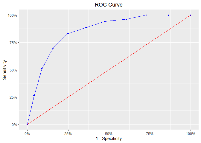
model %>%
  blr_gains_table() %>%
  blr_ks_chart()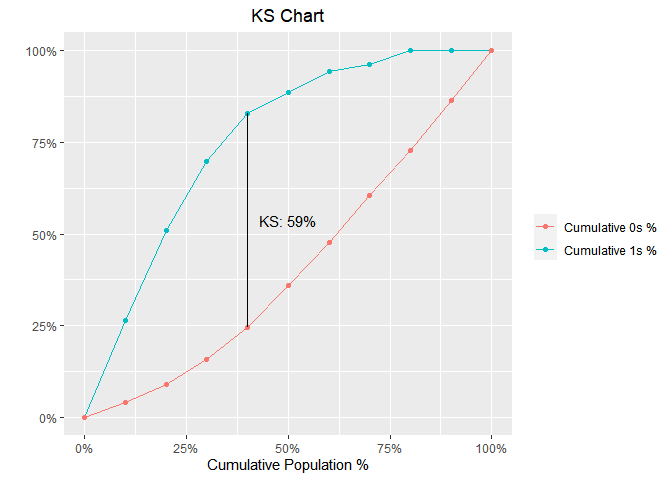
blr_lorenz_curve(model)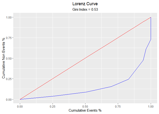
If you encounter a bug, please file a minimal reproducible example using reprex on github. For questions and clarifications, use StackOverflow.
These binaries (installable software) and packages are in development.
They may not be fully stable and should be used with caution. We make no claims about them.
Health stats visible at Monitor.