The hardware and bandwidth for this mirror is donated by dogado GmbH, the Webhosting and Full Service-Cloud Provider. Check out our Wordpress Tutorial.
If you wish to report a bug, or if you are interested in having us mirror your free-software or open-source project, please feel free to contact us at mirror[@]dogado.de.
Htmlwidget for billboard.js
![]()
![]()
This package allow you to use billboard.js, a re-usable easy interface JavaScript chart library, based on D3 v4+.
A proxy method is implemented to smoothly update charts in shiny applications, see below for details.
Install from CRAN with:
install.packages("billboarder")Install development version grom GitHub with:
# install.packages("remotes")
remotes::install_github("dreamRs/billboarder")
For interactive examples & documentation, see
pkgdown site :
https://dreamrs.github.io/billboarder/index.html
Simple bar chart :
library("billboarder")

# data
data("prod_par_filiere")

# a bar chart !
billboarder() %>%
  bb_barchart(data = prod_par_filiere[, c("annee", "prod_hydraulique")], color = "#102246") %>%
  bb_y_grid(show = TRUE) %>%
  bb_y_axis(tick = list(format = suffix("TWh")),
            label = list(text = "production (in terawatt-hours)", position = "outer-top")) %>%
  bb_legend(show = FALSE) %>%
  bb_labs(title = "French hydraulic production",
          caption = "Data source: RTE (https://opendata.rte-france.com)")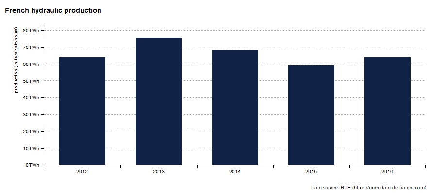
Multiple categories bar chart :
library("billboarder")

# data
data("prod_par_filiere")

# dodge bar chart !
billboarder() %>%
  bb_barchart(
    data = prod_par_filiere[, c("annee", "prod_hydraulique", "prod_eolien", "prod_solaire")]
  ) %>%
  bb_data(
    names = list(prod_hydraulique = "Hydraulic", prod_eolien = "Wind", prod_solaire = "Solar")
  ) %>%
  bb_y_grid(show = TRUE) %>%
  bb_y_axis(tick = list(format = suffix("TWh")),
            label = list(text = "production (in terawatt-hours)", position = "outer-top")) %>%
  bb_legend(position = "inset", inset = list(anchor = "top-right")) %>%
  bb_labs(title = "Renewable energy production",
          caption = "Data source: RTE (https://opendata.rte-france.com)")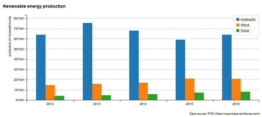
Stacked bar charts :
library("billboarder")

# data
data("prod_par_filiere")

# stacked bar chart !
billboarder() %>%
  bb_barchart(
    data = prod_par_filiere[, c("annee", "prod_hydraulique", "prod_eolien", "prod_solaire")],
    stacked = TRUE
  ) %>%
  bb_data(
    names = list(prod_hydraulique = "Hydraulic", prod_eolien = "Wind", prod_solaire = "Solar"),
    labels = TRUE
  ) %>%
  bb_colors_manual(
    "prod_eolien" = "#41AB5D", "prod_hydraulique" = "#4292C6", "prod_solaire" = "#FEB24C"
  ) %>%
  bb_y_grid(show = TRUE) %>%
  bb_y_axis(tick = list(format = suffix("TWh")),
            label = list(text = "production (in terawatt-hours)", position = "outer-top")) %>%
  bb_legend(position = "right") %>%
  bb_labs(title = "Renewable energy production",
          caption = "Data source: RTE (https://opendata.rte-france.com)")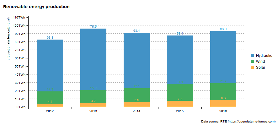
Classic :
library(billboarder)
library(palmerpenguins)
billboarder() %>%
  bb_scatterplot(data = penguins, x = "bill_length_mm", y = "flipper_length_mm", group = "species") %>%
  bb_axis(x = list(tick = list(fit = FALSE))) %>%
  bb_point(r = 8)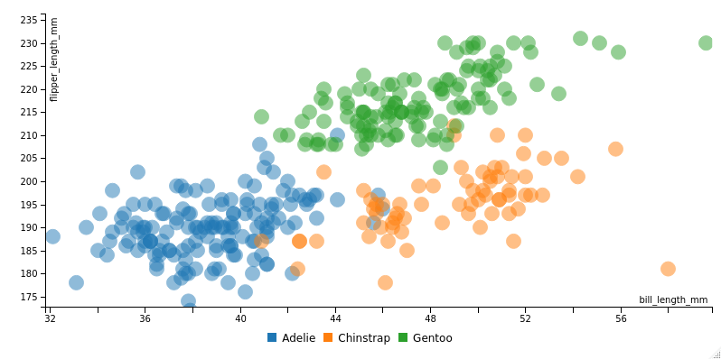
You can make a bubble chart using size aes :
billboarder() %>%
  bb_scatterplot(
    data = penguins,
    mapping = bbaes(
      bill_length_mm, flipper_length_mm, group = species,
      size = scales::rescale(body_mass_g, c(1, 100))
    )
  ) %>%
  bb_bubble(maxR = 25) %>%
  bb_x_axis(tick = list(fit = FALSE))
library("billboarder")

# data
data("prod_par_filiere")
nuclear2016 <- data.frame(
  sources = c("Nuclear", "Other"),
  production = c(
    prod_par_filiere$prod_nucleaire[prod_par_filiere$annee == "2016"],
    prod_par_filiere$prod_total[prod_par_filiere$annee == "2016"] -
      prod_par_filiere$prod_nucleaire[prod_par_filiere$annee == "2016"]
  )
)

# pie chart !
billboarder() %>%
  bb_piechart(data = nuclear2016) %>%
  bb_labs(title = "Share of nuclear power in France in 2016",
          caption = "Data source: RTE (https://opendata.rte-france.com)")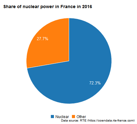
Date (and a subchart)library("billboarder")
# data
data("equilibre_mensuel")
# line chart
billboarder() %>%
bb_linechart(
data = equilibre_mensuel[, c("date", "consommation", "production")],
type = "spline"
) %>%
bb_x_axis(tick = list(format = "%Y-%m", fit = FALSE)) %>%
bb_x_grid(show = TRUE) %>%
bb_y_grid(show = TRUE) %>%
bb_colors_manual("consommation" = "firebrick", "production" = "forestgreen") %>%
bb_legend(position = "right") %>%
bb_subchart(show = TRUE, size = list(height = 30)) %>%
bb_labs(title = "Monthly electricity consumption and production in France (2007 - 2017)",
y = "In megawatt (MW)",
caption = "Data source: RTE (https://opendata.rte-france.com)")
billboarder() %>%
  bb_linechart(
    data = equilibre_mensuel[, c("date", "consommation", "production")],
    type = "spline"
  ) %>%
  bb_x_axis(tick = list(format = "%Y-%m", fit = FALSE)) %>%
  bb_x_grid(show = TRUE) %>%
  bb_y_grid(show = TRUE) %>%
  bb_colors_manual("consommation" = "firebrick", "production" = "forestgreen") %>%
  bb_legend(position = "right") %>%
  bb_zoom(
    enabled = TRUE,
    type = "drag",
    resetButton = list(text = "Unzoom")
  ) %>%
  bb_labs(title = "Monthly electricity consumption and production in France (2007 - 2017)",
          y = "In megawatt (MW)",
          caption = "Data source: RTE (https://opendata.rte-france.com)")
POSIXct (and regions)library("billboarder")
# data
data("cdc_prod_filiere")
# Retrieve sunrise and and sunset data with `suncalc`
library("suncalc")
sun <- getSunlightTimes(date = as.Date("2017-06-12"), lat = 48.86, lon = 2.34, tz = "CET")
# line chart
billboarder() %>%
bb_linechart(data = cdc_prod_filiere[, c("date_heure", "prod_solaire")]) %>%
bb_x_axis(tick = list(format = "%H:%M", fit = FALSE)) %>%
bb_y_axis(min = 0, padding = 0) %>%
bb_regions(
list(
start = as.numeric(cdc_prod_filiere$date_heure[1]) * 1000,
end = as.numeric(sun$sunrise)*1000
),
list(
start = as.numeric(sun$sunset) * 1000,
end = as.numeric(cdc_prod_filiere$date_heure[48]) * 1000
)
) %>%
bb_x_grid(
lines = list(
list(value = as.numeric(sun$sunrise)*1000, text = "sunrise"),
list(value = as.numeric(sun$sunset)*1000, text = "sunset")
)
) %>%
bb_labs(title = "Solar production (2017-06-12)",
y = "In megawatt (MW)",
caption = "Data source: RTE (https://opendata.rte-france.com)")
library("billboarder")

# data
data("cdc_prod_filiere")

# area chart !
billboarder() %>%
  bb_linechart(
    data = cdc_prod_filiere[, c("date_heure", "prod_eolien", "prod_hydraulique", "prod_solaire")],
    type = "area"
  ) %>%
  bb_data(
    groups = list(list("prod_eolien", "prod_hydraulique", "prod_solaire")),
    names = list("prod_eolien" = "Wind", "prod_hydraulique" = "Hydraulic", "prod_solaire" = "Solar")
  ) %>%
  bb_legend(position = "inset", inset = list(anchor = "top-right")) %>%
  bb_colors_manual(
    "prod_eolien" = "#238443", "prod_hydraulique" = "#225EA8", "prod_solaire" = "#FEB24C",
    opacity = 0.8
  ) %>%
  bb_y_axis(min = 0, padding = 0) %>%
  bb_labs(title = "Renewable energy production (2017-06-12)",
          y = "In megawatt (MW)",
          caption = "Data source: RTE (https://opendata.rte-france.com)")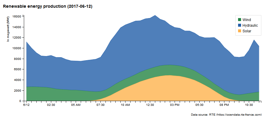
# Generate data
dat <- data.frame(
  date = seq.Date(Sys.Date(), length.out = 20, by = "day"),
  y1 = round(rnorm(20, 100, 15)),
  y2 = round(rnorm(20, 100, 15))
)
dat$ymin1 <- dat$y1 - 5
dat$ymax1 <- dat$y1 + 5

dat$ymin2 <- dat$y2 - sample(3:15, 20, TRUE)
dat$ymax2 <- dat$y2 + sample(3:15, 20, TRUE)


# Make chart : use ymin & ymax aes for range
billboarder(data = dat) %>%
  bb_linechart(
    mapping = bbaes(x = date, y = y1, ymin = ymin1, ymax = ymax1),
    type = "area-line-range"
  ) %>%
  bb_linechart(
    mapping = bbaes(x = date, y = y2, ymin = ymin2, ymax = ymax2),
    type = "area-spline-range"
  ) %>%
  bb_y_axis(min = 50)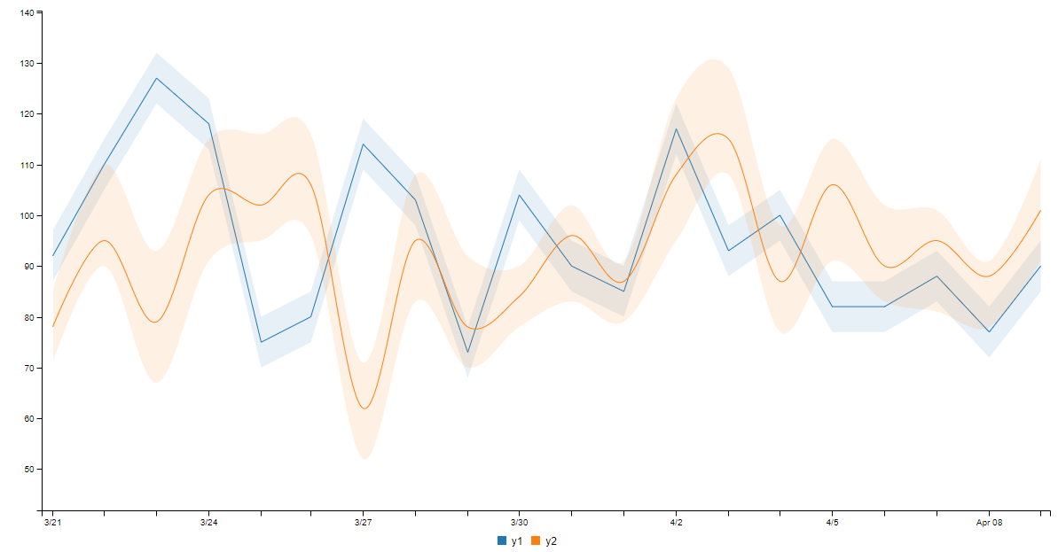
billboarder() %>%
  bb_histogram(data = rnorm(1e5), binwidth = 0.25) %>%
  bb_colors_manual()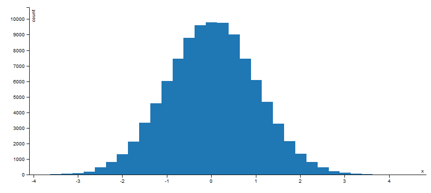
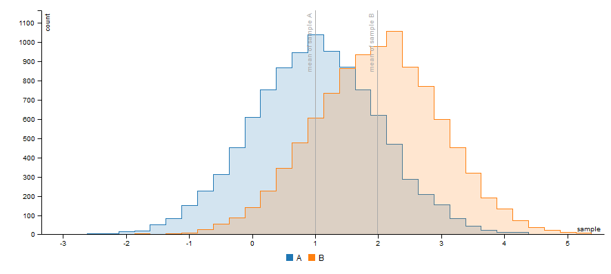
With a grouping variable :
# Generate some data
dat <- data.frame(
  sample = c(rnorm(n = 1e4, mean = 1), rnorm(n = 1e4, mean = 2)),
  group = rep(c("A", "B"), each = 1e4), stringsAsFactors = FALSE
)
# Mean by groups
samples_mean <- tapply(dat$sample, dat$group, mean)
# histogram !
billboarder() %>%
  bb_histogram(data = dat, x = "sample", group = "group", binwidth = 0.25) %>%
  bb_x_grid(
    lines = list(
      list(value = unname(samples_mean['A']), text = "mean of sample A"),
      list(value = unname(samples_mean['B']), text = "mean of sample B")
    )
  )
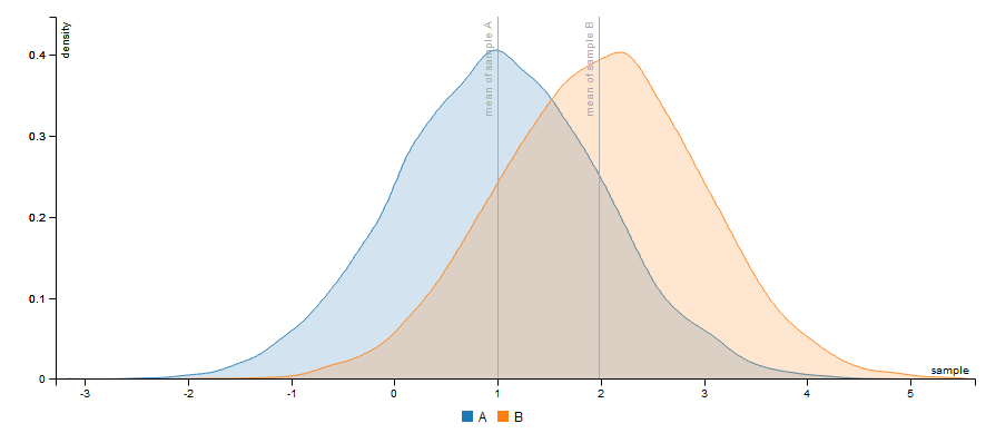
Density plot with the same data :
billboarder() %>%
  bb_densityplot(data = dat, x = "sample", group = "group") %>%
  bb_x_grid(
    lines = list(
      list(value = unname(samples_mean['A']), text = "mean of sample A"),
      list(value = unname(samples_mean['B']), text = "mean of sample B")
    )
  )
Some events will trigger Shiny’s inputs in application, such as
click. Inputs id associated with billboarder charts use
this pattern :
input$CHARTID_EVENTLook at this example, chart id is mybbchart so you
retrieve click with input$mybbchart_click :
library("shiny")
library("billboarder")

# data
data("prod_par_filiere")
prod_par_filiere_l <- reshape2::melt(data = prod_par_filiere)
prod_par_filiere_l <- prod_par_filiere_l[
  with(prod_par_filiere_l, annee == "2016" & variable != "prod_total"), 2:3
]
prod_par_filiere_l <- prod_par_filiere_l[order(prod_par_filiere_l$value), ]


# app
ui <- fluidPage(
  billboarderOutput(outputId = "mybbchart"),
  br(),
  verbatimTextOutput(outputId = "click")
)

server <- function(input, output, session) {

  output$mybbchart <- renderBillboarder({
    billboarder() %>%
      bb_barchart(data = prod_par_filiere_l) %>%
      bb_y_grid(show = TRUE) %>%
      bb_legend(show = FALSE) %>%
      bb_x_axis(categories = prod_par_filiere_l$variable, fit = FALSE) %>%
      bb_labs(title = "French electricity generation by branch in 2016",
              y = "production (in terawatt-hours)",
              caption = "Data source: RTE (https://opendata.rte-france.com)")
  })

  output$click <- renderPrint({
    cat("# input$mybbchart_click$category", "\n")
    input$mybbchart_click$category
  })

}

shinyApp(ui = ui, server = server)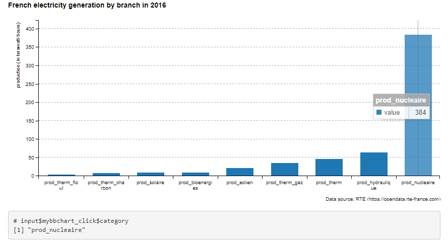
You can modify existing charts with function
billboarderProxy : 
To see examples, run :
library("billboarder")
proxy_example("bar")
proxy_example("line")
proxy_example("pie")
proxy_example("gauge")If you wish, you can build graphs using a list syntax
:
data(economics, package = "ggplot2")

# Construct a list in JSON format
params <- list(
  data = list(
    x = "x",
    json = list(
      x = economics$date,
      y = economics$psavert
    ),
    type = "spline"
  ),
  legend = list(show = FALSE),
  point = list(show = FALSE),
  axis = list(
    x = list(
      type = "timeseries",
      tick = list(
        count = 20,
        fit = TRUE,
        format = "%e %b %y"
      )
    ),
    y = list(
      label = list(
        text = "Personal savings rate"
      ),
      tick = list(
        format = htmlwidgets::JS("function(x) {return x + '%';}")
      )
    )
  )
)

# Pass the list as parameter
billboarder(params)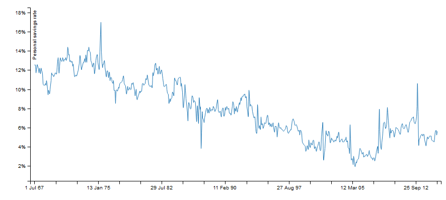
These binaries (installable software) and packages are in development.
They may not be fully stable and should be used with caution. We make no claims about them.
Health stats visible at Monitor.