The hardware and bandwidth for this mirror is donated by dogado GmbH, the Webhosting and Full Service-Cloud Provider. Check out our Wordpress Tutorial.
If you wish to report a bug, or if you are interested in having us mirror your free-software or open-source project, please feel free to contact us at mirror[@]dogado.de.
bayesestdft:
Estimating the degrees of freedom of the Student’s t-distribution
under a Bayesian frameworkSomjit Roy, Department of Statistics, Texas A&M University. Email: sroy_123@tamu.edu
Se Yoon Lee, Department of Statistics, Texas A&M University. Email: seyonlee.stat.math@gmail.com
bayesestdft is an R package providing tools to implement
Bayesian estimation of the degrees of
freedom in the Student’s t-distribution, that
are developed in Lee
(2022). Estimation experiments are run both on simulated as well as
real data, where broadly three Markov Chain Monte Carlo
(MCMC) sampling algorithms are used: (i) random
walk Metropolis (RMW), (ii)
Metropolis-adjusted Langevin Algorithm (MALA)
and (iii) Elliptical Slice Sampler (ESS)
respectively, to sample from the posterior distribution of the degrees
of freedom.
The current version of the package bayesestdft 1.0.0
provides Bayesian routines to estimate the degrees of freedom of the
Student’s t-distribution with Jeffreys prior
(BayesJeffreys), Gamma prior
(BayesGA), and Log-normal prior
(BayesLNP) endowed upon as the prior distribution over the
degrees of freedom. MALA is used to draw posterior
samples in case of the Jeffreys prior, hence to operate the function
BayesJeffreys, the user needs to install the
numDeriv R package. For more technical insights into
bayesestdft, refer to the slides.
bayesestdftbayesestdft.numDeriv and
dplyr.Now bayesestdft can be installed from both
Github and CRAN respectively, using
the following lines of code:
library(devtools)
devtools::install_github("Roy-SR-007/bayesestdft")
library(bayesestdft)install.packages("bayesestdft")
library(bayesestdft)bayesestdft facilitates a full Bayesian
framework for the estimation of the
degrees of freedom in the Student’s
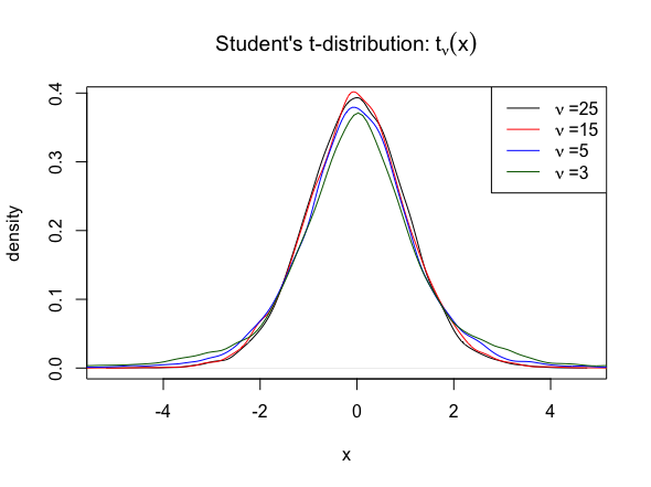
t-distribution. More precisely, given \(N\) independent and identical samples \(x = (x_1,x_2, \cdots, x_N)\) from the
Student’s t-distribution:
\[ t_{\nu}(x) = \frac{\Gamma\left( \frac{\nu+1}{2} \right)}{\sqrt{\nu \pi} \Gamma\left( \frac{\nu}{2} \right)} \left(1 + \frac{x^2}{\nu} \right)^{-\frac{\nu +1}{2}}, \quad x \in \mathbb{R} \]

and a prior distribution \(\pi(\nu)\) over the degrees of freedom \(\nu\), the aim is to sample from the posterior distribution:
\[ \pi(\nu|\textbf{x}) = \frac{\left[\prod_{i=1}^{N} t_{\nu}(x_i) \right]\cdot \pi(\nu)}{\int_{\mathbb{R}^{+}} \left[\prod_{i=1}^{N} t_{\nu}(x_i)\right] \cdot \pi(\nu) d\nu}, \quad \nu \in \mathbb{R}^+ \]
The current version of the package bayesestdft 1.0.0,
provides four prior choices \(\pi(\nu)\) viz., the
Jeffreys prior \(\pi_J(\nu)\), an
exponential prior \(\pi_E(\nu)\), a gamma
prior \(\pi_G(\nu)\), and a
log-normal prior \(\pi_L(\nu)\).
\[ \pi_{J}(\nu) \propto \left(\frac{\nu}{\nu+3} \right)^{1/2} \left( \psi'\left(\frac{\nu}{2}\right) -\psi'\left(\frac{\nu+1}{2}\right) -\frac{2(\nu + 3)}{\nu(\nu+1)^2}\right)^{1/2},\quad \nu \in \mathbb{R}^+\]
where \(\psi(a) =
\frac{d\log\Gamma(a)}{da}\) and \(\psi'(a) = \frac{d\Psi(a)}{da}\) are
the digamma and trigamma functions
respectively, which are computed using the R functions
digamma() and trigamma() in the
base package.
BayesJeffreysWe consider \(N=100\) simulated
observations \(x = (x_1, x_2, \cdot,
x_N)\) from \(t_{0.1}\)
distribution, where the degrees of freedom is \(\nu = 0.1\). We estimate \(\nu\) using the Jeffreys
prior and consider posterior samples from both RMW and
MALA MCMC sampling engines. The corresponding R code
for using the function BayesJeffreys() to sample from the
posterior with a Jeffreys prior over the degrees of
freedom \(\nu\) is:
x = rt(n = 100, df = 0.1)

# simulating S = 10000 posterior samples
nu1 = BayesJeffreys(x, S = 10000, sampling.alg = "MH")
nu2 = BayesJeffreys(x, S = 10000, sampling.alg = "MALA")
# posterior mean estimate from the RMW algorithm
mean(nu1)
# posterior mean estimate from the MALA sampling scheme
mean(nu2)
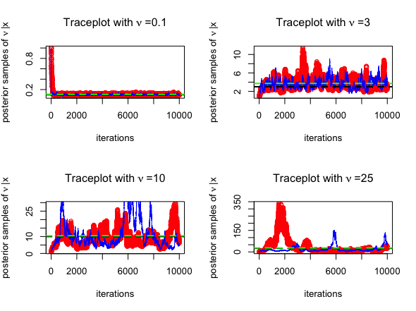
The trace plots for MCMC algorithms (posterior samples obtained from RWM in red and those obtained from MALA in blue) are given below, for \(\nu = 0.1, 3, 10, 25\). The posterior mean is highlighted in green below.
\[ \pi_{E}(\nu) =Ga(\nu|1,0.1) = Exp(\nu|0.1) = \frac{1}{10} e^{-\nu/10},\quad \nu \in \mathbb{R}^+\]
where the rate hyper-parameter has been set to \(0.1\) following Fernández and Steel (1998).
BayesGAOnce again, we consider \(N=100\)
simulated observations \(x = (x_1, x_2, \cdot,
x_N)\) from \(t_{0.1}\)
distribution, where the degrees of freedom is \(\nu = 0.1\). We estimate \(\nu\) using the
Exponential prior and consider posterior samples from
RMW MCMC scheme. Following is the R code for using the
function BayesGA():
x = rt(n = 100, df = 0.1)

# simulating S = 10000 posterior samples
nu = BayesGA(x, S = 10000, a = 1, b = 0.1)
# posterior mean estimate
mean(nu)
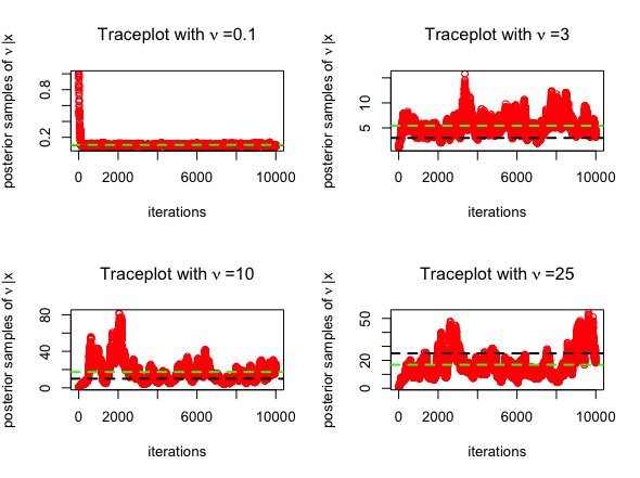
The trace plots for MCMC algorithm (posterior samples obtained from RWM in red) are given below, for \(\nu = 0.1, 3, 10, 25\). The posterior mean is highlighted in green below.
\[ \pi_{G}(\nu) =Ga(\nu|2,0.1) =\frac{\nu}{100} e^{-\nu/10},\quad \nu \in \mathbb{R}^+\]
where the shape and rate hyper-parameters are set to \(2\) and \(0.1\) respectively, as recommended by Juárez and Steel (2010).
BayesGAThe BayesGA() function is implemented with the same
configuration as above in case of the Exponential prior
with a slight generalization of inducing a Gamma prior
over \(\nu\). To what follows, is the R
code for using BayesGA() under the Gamma prior set up with
posterior sampling being done using the RWM scheme:
x = rt(n = 100, df = 0.1)

# simulating S = 10000 posterior samples
nu = BayesGA(x, S = 10000, a = 2, b = 0.1)
# posterior mean estimate
mean(nu)
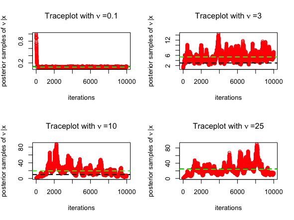
The trace plots for MCMC algorithm (posterior samples obtained from RWM in red) are given below, for \(\nu = 0.1, 3, 10, 25\). The posterior mean is highlighted in green below.
The Log-normal prior has been suggested as a viable option in Lee (2022) with the choice of mean and variance hyper-parameters as \(1\), a justification to which has been provided through the sensitivity analysis done in Section 4.1 of Lee (2022).
\[ \pi_{L}(\nu) =logN(\nu|1,1) =\frac{1}{\nu \sqrt{2\pi}} \exp\left[- \frac{(\log \nu - 1)^2}{2} \right],\quad \nu \in \mathbb{R}^+\]
BayesLNPThe BayesLNP() function draws posterior samples using
the Elliptical Slice Sampler (ESS),
considering a Log-normal prior over the degrees of
freedom \(\nu\), and the R code for its
implementation is given below:
x = rt(n = 100, df = 0.1)

# simulating S = 10000 posterior samples
nu = BayesLNP(x, S = 10000)
# posterior mean estimate
mean(nu)
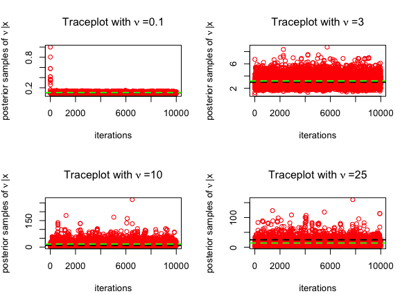
The trace plots for MCMC algorithm (posterior samples obtained from ESS in red) are given below, for \(\nu = 0.1, 3, 10, 25\). The posterior mean is highlighted in green below.
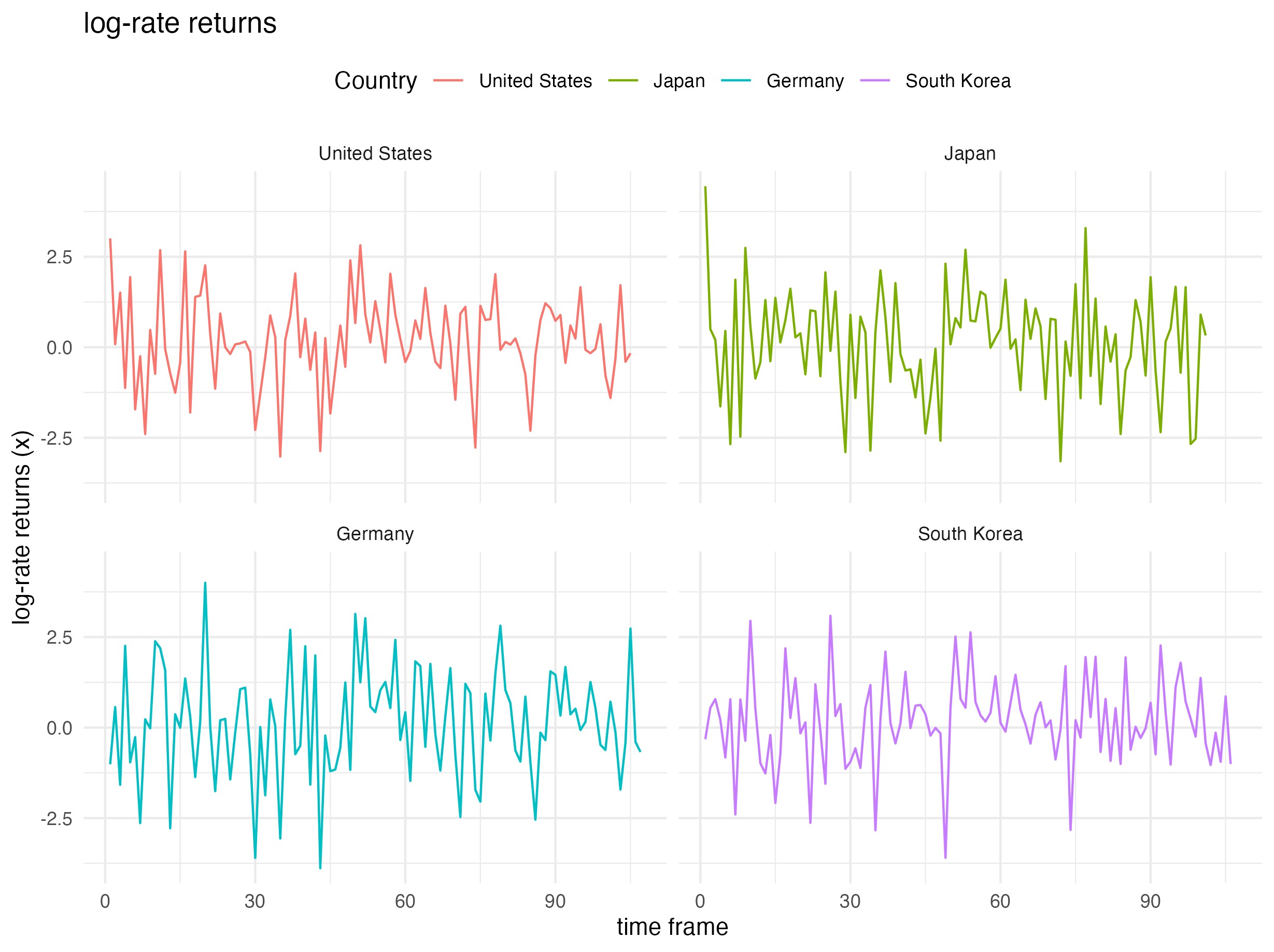
Heavy-tailed daily stock return index values were considered for four countries: (i) United States (S&P500), (ii) Japan (NIKKEI225), (iii) Germany (DAX Index), and (iv) South Korea (KOSPI). Particularly, the data of United States (S&P500) from June 02, 2009 through October 30, 2009 is picked up for analysis resulting into a sample size of \(N = 100\) observations.
The log-rate returns (multiplied by \(100\)): \(x_i = \log\left(X_{i+1}/X_{i}\right)\times 100\) is modeled, where \(x_i\) is assumed to be Student’s t-distributed and \(X_i\) denotes the market index on the \(i\)-th trading day. The plot below shows the country-specific \(x_i\)’s.
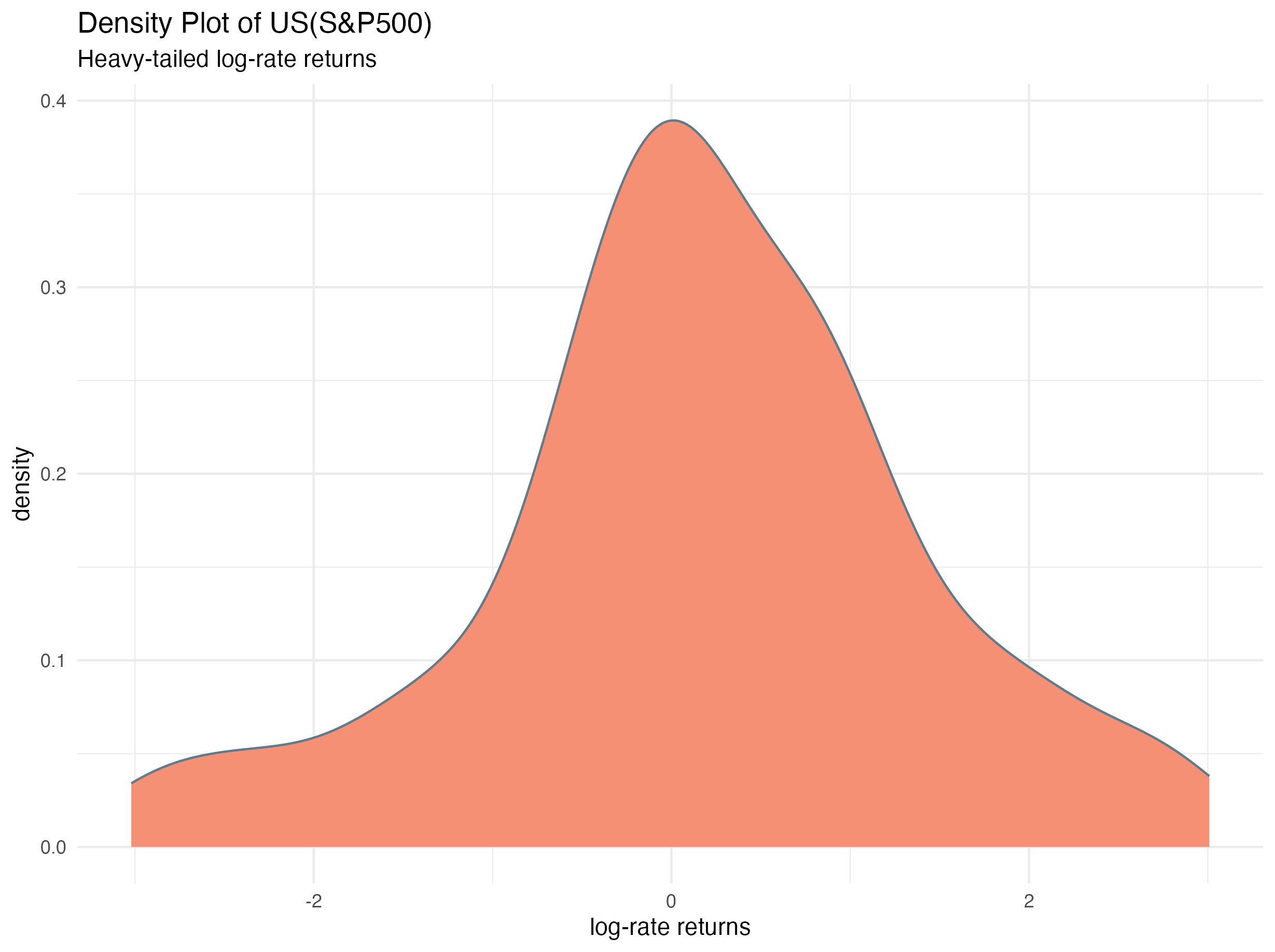
The density plot of the log-rate returns for United States (S&P500) illustrating the heavy-tailed nature of the observations is given below:
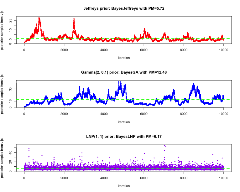
We considering running the (i) MALA sampler for the
Jeffreys prior over \(\nu\), i.e., using
BayesJeffreys for sampling \(S=10000\) posterior samples, (ii)
RWM algorithm for the Gamma prior over
\(\nu\) (with shape and rate
hyper-parameters specified as, \(2\)
and \(0.1\) respectively), i.e., using
BayesGA for sampling \(S=10000\) posterior samples, and (iii)
ESS algorithm for the Log-normal prior
over \(\nu\) (with mean and variance
hyper-parameters specified as \(1\)),
i.e., using BayesLNP for sampling \(S=10000\) posterior samples.
library(dplyr)

# loading the log-rate returns data
data(index_return)

# filtering out the data specific to United States (S&P500)
index_return_US <- filter(index_return, Country == "United States")
x = index_return_US$log_return_rate

# Jeffreys prior over the degrees of freedom
nu_jeffreys = BayesJeffreys(x, S = 10000, sampling.alg = "MALA")
# posterior mean (pm) estimate
nu_jeffreys_pm = mean(nu_jeffreys)

# Gamma prior over the degrees of freedom
nu_gamma = BayesGA(x, S = 10000, a = 2, b = 0.1)
# posterior mean (pm) estimate
nu_gamma_pm = mean(nu_gamma)

# Log-normal prior over the degrees of freedom
nu_LNP = BayesLNP(x, S = 10000)
# posterior mean (pm) estimate
nu_LNP_pm = mean(nu_LNP)
The trace plots of the posterior samples are given below, for different choices of priors as employed above. The posterior mean estimate of the degrees of freedom is also highlighted in each of the cases.
[1] Lee, S. Y. (2022). The Use of a Log-Normal Prior for the Student t-Distribution. Axioms, 11(9), 462. https://doi.org/10.3390/axioms11090462.
These binaries (installable software) and packages are in development.
They may not be fully stable and should be used with caution. We make no claims about them.
Health stats visible at Monitor.