The hardware and bandwidth for this mirror is donated by dogado GmbH, the Webhosting and Full Service-Cloud Provider. Check out our Wordpress Tutorial.
If you wish to report a bug, or if you are interested in having us mirror your free-software or open-source project, please feel free to contact us at mirror[@]dogado.de.
![]()
![]()
The goal of ameras is to provide a user-friendly interface to analyze association studies with multiple realizations of a noisy exposure using a variety of methods. ameras supports continuous, count, binary, multinomial, and right-censored time-to-event outcomes. For binary outcomes, the nested case-control design is also accommodated. Besides the common exponential relative risk model \(RR=\exp(\beta D)\) for the exposure-outcome association with noisy exposure \(D\), linear excess relative risk \(RR=1+\beta D\) and linear-exponential excess relative risk models \(RR=1+\beta_1 D \exp(\beta_2 D)\) can be used.
To install from CRAN:
install.packages("ameras")To install the development version from GitHub:
# install.packages("pak") # If pak is not already installed
pak::pak("sanderroberti/ameras")This is a basic example which shows you how to fit a simple logistic regression model. First, we visualize the dose uncertainty. In the left panel of the plot below, the empirical cumulative distribution function (ECDF) is plotted for each dose realization. In other words, each curve shows one distribution of dose across individuals. The spread within individual curves reflects the dose range across individuals, while the spread between curves reflects between-realization variation on the cohort level.
In the right panel, ECDFs are plotted for each individual, showing distributions within individuals. A wide spread within individual curves is indicative of large within-individual variation, while the spread between curves reflects between-individual variation.
library(ameras)
#> Loading required package: nimble
#> nimble version 1.4.2 is loaded.
#> For more information on NIMBLE and a User Manual,
#> please visit https://R-nimble.org.
#>
#> Attaching package: 'nimble'
#> The following object is masked from 'package:stats':
#>
#>     simulate
#> The following object is masked from 'package:base':
#>
#>     declare
data(data, package="ameras")
ecdfplot(data, paste0("V", 1:10), show.mean = FALSE)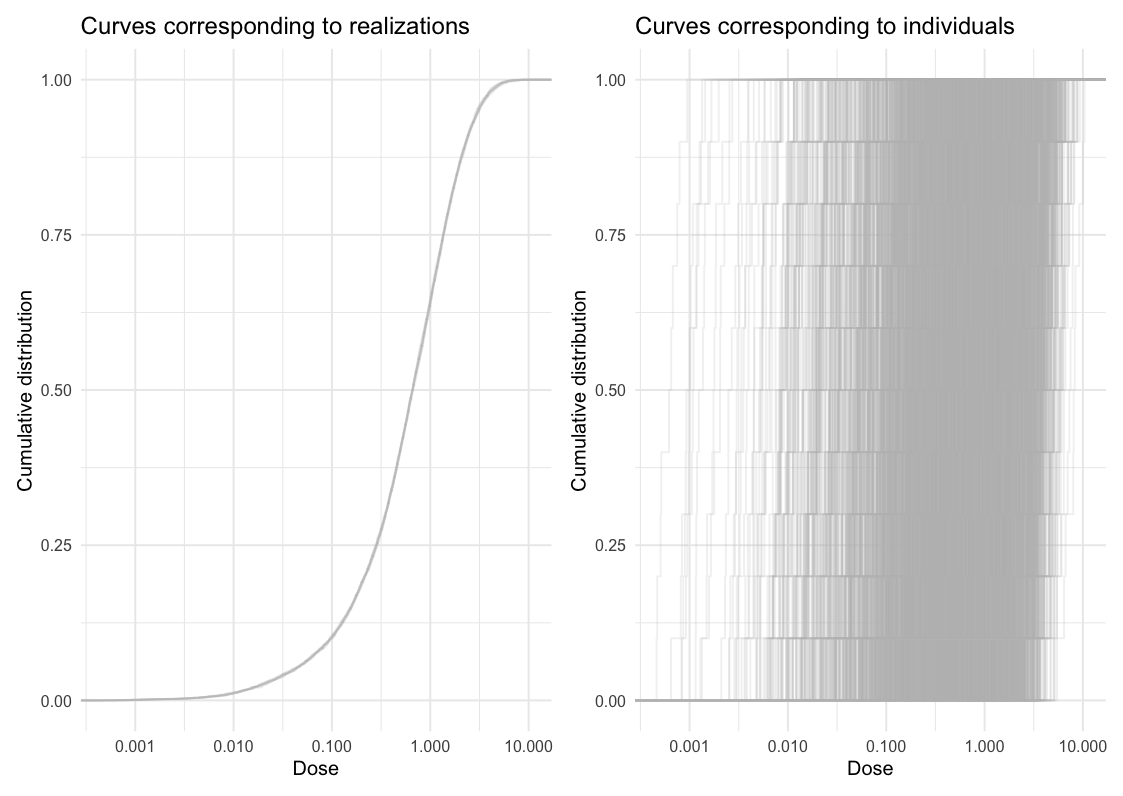
Next, we apply all available methods to the data:
set.seed(12345) # For reproducibility
fit <- ameras(Y.binomial~dose(V1:V10), data, family="binomial",
              methods=c("RC","ERC","MCML", "FMA", "BMA"))
#> Note: BMA may require extensive computation time
#> Fitting RC
#> Fitting ERC
#> Fitting MCML
#> Fitting FMA
#> Fitting BMA
#> Defining model
#> Building model
#> Setting data and initial values
#> Running calculate on model
#>   [Note] Any error reports that follow may simply reflect missing values in model variables.
#> Checking model sizes and dimensions
#>   [Note] This model is not fully initialized. This is not an error.
#>          To see which variables are not initialized, use model$initializeInfo().
#>          For more information on model initialization, see help(modelInitialization).
#> Compiling
#>   [Note] This may take a minute.
#>   [Note] Use 'showCompilerOutput = TRUE' to see C++ compilation details.
#> Compiling
#>   [Note] This may take a minute.
#>   [Note] Use 'showCompilerOutput = TRUE' to see C++ compilation details.
#> running chain 1...
#> |-------------|-------------|-------------|-------------|
#> |-------------------------------------------------------|
#> running chain 2...
#> |-------------|-------------|-------------|-------------|
#> |-------------------------------------------------------|
summary(fit)
#> Call:
#> ameras(formula = Y.binomial ~ dose(V1:V10), data = data, family = "binomial",
#>     methods = c("RC", "ERC", "MCML", "FMA", "BMA"))
#>
#> Rows: 3000
#>
#> Total CPU runtime: 51.2 seconds
#>
#> CPU runtime in seconds by method:
#>
#>  Method    Fit  CI  Total
#>      RC  0.028 0.0  0.028
#>     ERC  7.951 0.0  7.951
#>    MCML  0.110 0.0  0.110
#>     FMA  0.311 0.0  0.311
#>     BMA 42.780 0.0 42.780
#>
#> Summary of coefficients by method:
#>
#>  Method        Term Estimate      SE Rhat   n.eff
#>      RC (Intercept)  -0.8847 0.07378   NA      NA
#>      RC        dose   0.8020 0.13751   NA      NA
#>     ERC (Intercept)  -0.8849 0.07477   NA      NA
#>     ERC        dose   0.8214 0.14304   NA      NA
#>    MCML (Intercept)  -0.8758 0.07323   NA      NA
#>    MCML        dose   0.7910 0.13644   NA      NA
#>     FMA (Intercept)  -0.8760 0.07320   NA      NA
#>     FMA        dose   0.7917 0.13656   NA      NA
#>     BMA (Intercept)  -0.8736 0.07174 1.00 1024.00
#>     BMA        dose   0.7911 0.13323 1.00  999.00
#>
#> Note: confidence intervals not yet computed. Use confint() to add them.
Finally, we add confidence intervals to the fit
object:
fit <- confint(fit, type=c("wald.orig","percentile"))
#> RC confidence intervals:
#>
#> lower upper
#> (Intercept) -1.0293 -0.7401
#> dose 0.5324 1.0715
#>
#> ERC confidence intervals:
#>
#> lower upper
#> (Intercept) -1.0314 -0.7384
#> dose 0.5411 1.1018
#>
#> MCML confidence intervals:
#>
#> lower upper
#> (Intercept) -1.0193 -0.7323
#> dose 0.5236 1.0584
#>
#> FMA confidence intervals:
#>
#> lower upper
#> (Intercept) -1.0199 -0.7327
#> dose 0.5241 1.0594
#>
#> BMA confidence intervals:
#>
#> lower upper
#> (Intercept) -1.019 -0.735
#> dose 0.552 1.080
summary(fit)
#> Call:
#> ameras(formula = Y.binomial ~ dose(V1:V10), data = data, family = "binomial",
#> methods = c("RC", "ERC", "MCML", "FMA", "BMA"))
#>
#> Rows: 3000
#>
#> Total CPU runtime: 51.2 seconds
#>
#> CPU runtime in seconds by method:
#>
#> Method Fit CI Total
#> RC 0.028 0.001 0.029
#> ERC 7.951 0.000 7.951
#> MCML 0.110 0.000 0.110
#> FMA 0.311 0.004 0.315
#> BMA 42.780 0.001 42.781
#>
#> Summary of coefficients by method:
#>
#> Method Term Estimate SE CI.lower CI.upper Rhat n.eff
#> RC (Intercept) -0.8847 0.07378 -1.0293 -0.7401 NA NA
#> RC dose 0.8020 0.13751 0.5324 1.0715 NA NA
#> ERC (Intercept) -0.8849 0.07477 -1.0314 -0.7384 NA NA
#> ERC dose 0.8214 0.14304 0.5411 1.1018 NA NA
#> MCML (Intercept) -0.8758 0.07323 -1.0193 -0.7323 NA NA
#> MCML dose 0.7910 0.13644 0.5236 1.0584 NA NA
#> FMA (Intercept) -0.8760 0.07320 -1.0199 -0.7327 NA NA
#> FMA dose 0.7917 0.13656 0.5241 1.0594 NA NA
#> BMA (Intercept) -0.8736 0.07174 -1.0185 -0.7350 1.00 1024.00
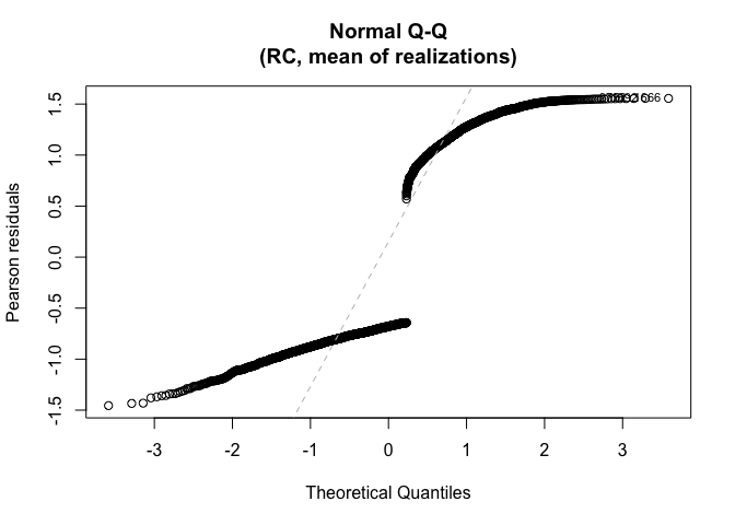
#> BMA dose 0.7911 0.13323 0.5520 1.0798 1.00 999.00For visual model diagnostics using residuals, use
plot(). For example, for regression calibration:
plot(fit, methods="RC")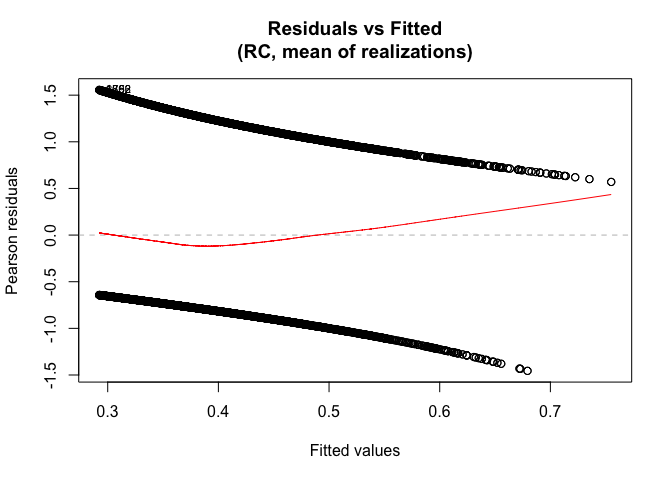
See the vignettes for additional details on model fitting, confidence intervals, transformations, standard analyses with one dose realization, manual FMA through multiple RC fits, and parallel FMA.
These binaries (installable software) and packages are in development.
They may not be fully stable and should be used with caution. We make no claims about them.
Health stats visible at Monitor.