The hardware and bandwidth for this mirror is donated by dogado GmbH, the Webhosting and Full Service-Cloud Provider. Check out our Wordpress Tutorial.
If you wish to report a bug, or if you are interested in having us mirror your free-software or open-source project, please feel free to contact us at mirror[@]dogado.de.

adass

The package adass implements the adaptive smoothing spline (AdaSS) estimator for the function-on-function linear regression model proposed by Centofanti et al. (2023). The AdaSS estimator is obtained by the optimization of an objective function with two spatially adaptive penalties, based on initial estimates of the partial derivatives of the regression coefficient function. This allows the proposed estimator to adapt more easily to the true coefficient function over regions of large curvature and not to be undersmoothed over the remaining part of the domain. The package comprises two main functions adass.fr and adass.fr_eaass. The former implements the AdaSS estimator for fixed tuning parameters. The latter executes the evolutionary algorithm for the adaptive smoothing spline estimator (EAASS) algorithm to select the optimal tuning parameter combination as described in Centofanti et al. (2023).

Installation

You can install the released version of adass from CRAN with:

install.packages("adass")

The development version can be installed from GitHub with:

# install.packages("devtools")
devtools::install_github("unina-sfere/adass")

Example

This is a basic example which shows you how to apply the two main functions adass.fr and adass.fr_eaass on a synthetic dataset generated as described in the simulation study of Centofanti et al. (2023).

We start by loading and attaching the adass package.

library(adass)

Then, we generate the synthetic dataset and build the basis function sets as follows.

case<-"Scenario HAT"
data<-simulate_data(case,n_obs=10)
X_fd <- data$X_fd
Y_fd <- data$Y_fd
basis_s <- fda::create.bspline.basis(c(0,1),nbasis = 30,norder = 4)
basis_t <- fda::create.bspline.basis(c(0,1),nbasis = 30,norder = 4)

Then, we calculate the initial estimate of the partial derivatives of the coefficient function.

mod_smooth <-adass.fr(Y_fd,X_fd,basis_s = basis_s,basis_t = basis_t,tun_par=c(10^-6,10^-6,0,0,0,0))
grid_s<-seq(0,1,length.out = 10)
grid_t<-seq(0,1,length.out = 10)
beta_der_eval_s<-fda::eval.bifd(grid_s,grid_t,mod_smooth$Beta_hat_fd,sLfdobj = 2)
beta_der_eval_t<-fda::eval.bifd(grid_s,grid_t,mod_smooth$Beta_hat_fd,tLfdobj = 2) 

Then, we apply the EAASS algorithm through the adass.fr_eaass function to identify the optimal combination of tuning parameters.

mod_adass_eaass<-adass.fr_eaass(Y_fd,X_fd,basis_s,basis_t,
                      beta_ders=beta_der_eval_s, beta_dert=beta_der_eval_t,
                      rand_search_par=list(c(-8,4),c(-8,4),c(0,0.1),c(0,4),c(0,0.1),c(0,4)),
                      grid_eval_ders=grid_s,grid_eval_dert=grid_t,
                      popul_size = 10,ncores=8,iter_num=5)

Finally, adass.fr is applied with tuning parameters fixed to their optimal values.

mod_adass <-adass.fr(Y_fd, X_fd, basis_s = basis_s, basis_t = basis_t,
                   tun_par=mod_adass_eaass$tun_par_opt,beta_ders = beta_der_eval_s,
                   beta_dert = beta_der_eval_t,grid_eval_ders=grid_s,grid_eval_dert=grid_t )

The resulting estimator is plotted as follows.

plot(mod_adass)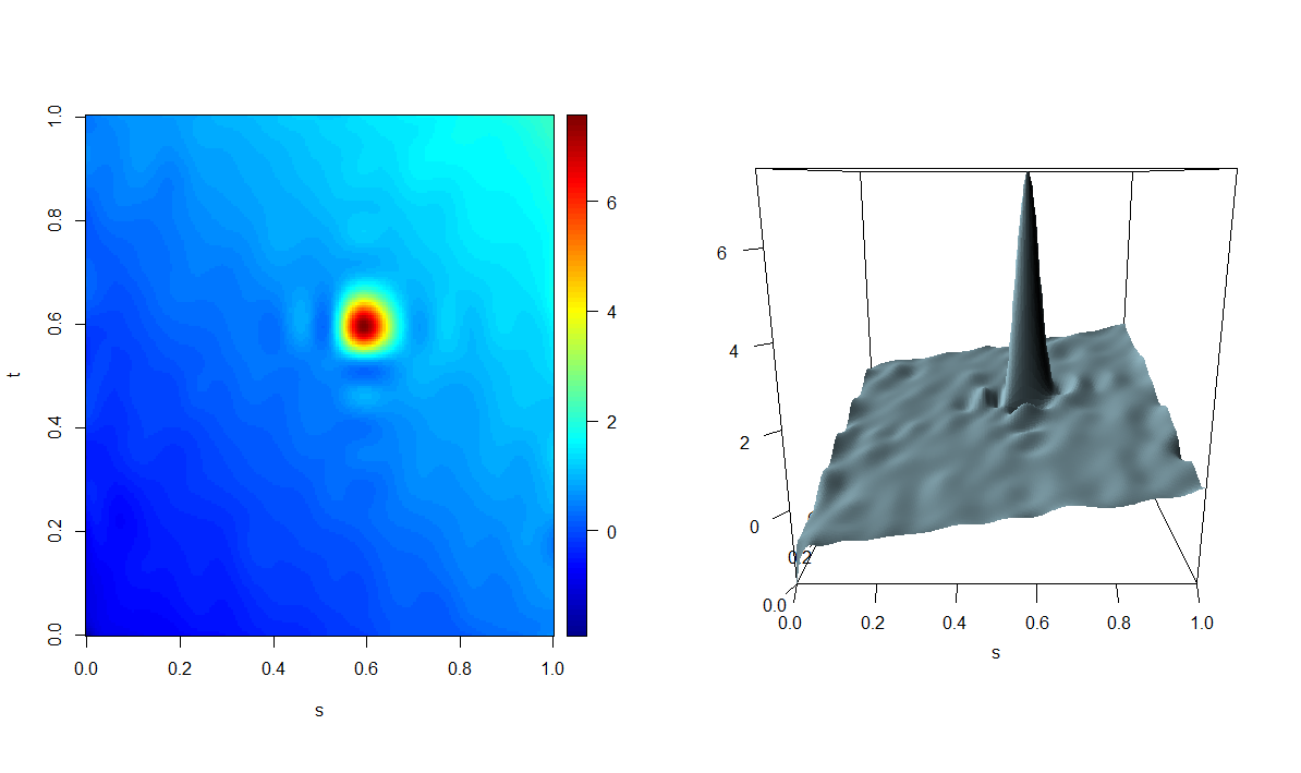

References

• Centofanti, F., Lepore, A., Menafoglio, A., Palumbo, B., Vantini, S. (2023). Adaptive Smoothing Spline Estimator for the Function-on-Function Linear Regression Model. Computational Statistics 38(1), 191–216.

These binaries (installable software) and packages are in development.
They may not be fully stable and should be used with caution. We make no claims about them.
Health stats visible at Monitor.