The hardware and bandwidth for this mirror is donated by dogado GmbH, the Webhosting and Full Service-Cloud Provider. Check out our Wordpress Tutorial.
If you wish to report a bug, or if you are interested in having us mirror your free-software or open-source project, please feel free to contact us at mirror[@]dogado.de.
The goal of abima is to assess whether and how a specific continuous or categorical exposure affects the outcome of interest through one- or multi-dimensional mediators using an adaptive bootstrap (AB) approach. The AB method allows to make inference for composite null hypotheses of no mediation effect, providing valid type I error control and thus optimizes statistical power. For more technical details, refer to He, Y., Song, P. X. K., and Xu, G. (2023), “Adaptive bootstrap tests for composite null hypotheses in the mediation pathway analysis,” Journal of the Royal Statistical Society Series B: Statistical Methodology, qkad129. https://doi.org/10.1093/jrsssb/qkad129.
Install the R CRAN version of abima like so:
install.packages("abima")or install the development version of abima like so:
# Install abima from GitHub:
devtools::install_github("canyi-chen/abima")This is a single example that shows steps of using the adaptive bootstrap (AB) to test for the null hypothesis of no mediation effect under the linear structral equation models.
library(abima)


## Set up parameters
alpha_S <- beta_M <- 1/6

set.seed(2)
data <- generate_all_data(
  n = 200,
  alpha_S = alpha_S,
  beta_M = beta_M
)
S <- data$S
M <- data$M
Y <- data$Y
X <- data$X

abYlm.Mlm(
  S,
  M,
  Y,
  X,
  B = 199
)
#> $NIE
#> [1] 0.03081102
#>
#> $p_value_NIE
#> [1] 0.01507538
#>
#> $NDE
#> [1] 1.034168
#>
#> $p_value_NDE
#> [1] 2.535113e-31
#>
#> $NTE
#> [1] 1.064979
#>
#> $p_value_NTE
#> [1] 7.724359e-34
#>
#> attr(,"class")
#> [1] "abYlmMlmResult"library(abima)
## Set up parameters
alpha_S <- beta_M <- rep(1/6, 2)
set.seed(2)
data <- generate_all_data(
n = 200,
alpha_S = alpha_S,
beta_M = beta_M
)
S <- data$S
M <- data$M
Y <- data$Y
X <- data$X
abYlm.Mlm(
S,
M,
Y,
X,
B = 199
)
#> $NIE
#> [1] 0.03820384
#>
#> $p_value_NIE
#> [1] 0.005025126
#>
#> $NDE
#> [1] 1.072573
#>
#> $p_value_NDE
#> [1] 2.063533e-33
#>
#> $NTE
#> [1] 1.110776
#>
#> $p_value_NTE
#> [1] 2.829119e-37
#>
#> attr(,"class")
#> [1] "abYlmMlmResult"This example shows the use of abYlm.Mglm function with confounders covariates_cfder being included in the mediation analysis.
library(abima)


## Set up parameters
M.family <- poisson()
alpha_S <- beta_M <- 1/15

set.seed(2)
data <- generate_all_data(
  n = 200,
  alpha_S = alpha_S,
  beta_M = beta_M,
  M.family = M.family
)
S <- data$S
M <- data$M
Y <- data$Y
X <- data$X

abYlm.Mglm(
  S,
  M,
  Y,
  X,
  M.family = M.family,
  B = 199
)
#> $NIE
#> [1] 0.02642484
#>
#> $p_value_NIE
#> [1] 0.01005025
#>
#> $NDE
#> [1] 1.016851
#>
#> $p_value_NDE
#> [1] 4.579245e-32
#>
#> $NTE
#> [1] 1.043276
#>
#> $p_value_NTE
#> [1] 0
#>
#> attr(,"class")
#> [1] "abYlmMglmResult"

abYlm.Mglm(
  S,
  M,
  Y,
  X,
  covariates_cfder = colMeans(X), # the covariates_cfder that you would to condition on
  M.family = M.family,
  B = 199
)
#> $NIE
#> [1] 0.03110028
#>
#> $p_value_NIE
#> [1] 0.01005025
#>
#> $NDE
#> [1] 1.016851
#>
#> $p_value_NDE
#> [1] 4.579245e-32
#>
#> $NTE
#> [1] 1.047951
#>
#> $p_value_NTE
#> [1] 0
#>
#> attr(,"class")
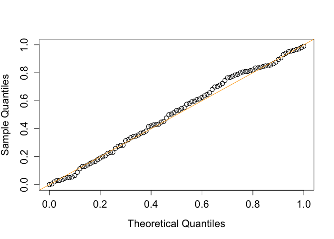
#> [1] "abYlmMglmResult"This exmaple shows that the performance of adaptive bootstrap test in the type I error control under the composite null hypothesis.
## Load libraries
library(abima)

if (rlang::is_installed("future.apply")) {
  library(future.apply)
  plan(multisession, workers = 12)
} else {
  install.packages("future.apply")
  library(future.apply)
  plan(multisession, workers = 12)
}
#> Loading required package: future


## Set up parameters
M.family <- gaussian()
Y.family <- gaussian()

simulation <- function(alpha_S = 0, beta_M = 0) {
  data <- generate_all_data(
    n = 500,
    alpha_S = alpha_S,
    beta_M = beta_M,
    M.family = M.family,
    Y.family = Y.family
  )
  S <- data$S
  M <- data$M
  Y <- data$Y
  X <- data$X

  out <- abYlm.Mlm(
    S,
    M,
    Y,
    X,
    B = 199
  )
  out
}


## Empirical distribution of the p value
# the number of replication for approximating the distribution of the p value
Nreps <- 200
alpha_S <- beta_M <- 0
output <- future_replicate(Nreps, simulation(0, 0))


plot(
  seq(0, 1, 0.01),
  quantile(unlist(output[2,]), probs = seq(0, 1, 0.01)),
  pch = 1,
  cex = 1.2,
  cex.lab = 1.3,
  cex.axis = 1.3,
  ylab = "Sample Quantiles",
  xlab = "Theoretical Quantiles",
  type = "p",
  xlim = c(0, 1),
  ylim = c(0, 1),
  lwd = 1.2
)
abline(0, 1, col = "orange")
These binaries (installable software) and packages are in development.
They may not be fully stable and should be used with caution. We make no claims about them.
Health stats visible at Monitor.