The hardware and bandwidth for this mirror is donated by dogado GmbH, the Webhosting and Full Service-Cloud Provider. Check out our Wordpress Tutorial.
If you wish to report a bug, or if you are interested in having us mirror your free-software or open-source project, please feel free to contact us at mirror[@]dogado.de.
We provide R code for Zero-inflated Poisson-Gamma Model (ZIPG) with an application to longitudinal microbiome count data.
You can install the development version of ZIPG like so:
devtools::install_github("roulan2000/ZIPG")Load dietary data. Complete Dietary data can be found in “Daily sampling reveals personalized diet-microbiome associations in humans.” (Johnson et al. 2019)
library(ZIPG)
library(ggplot2)
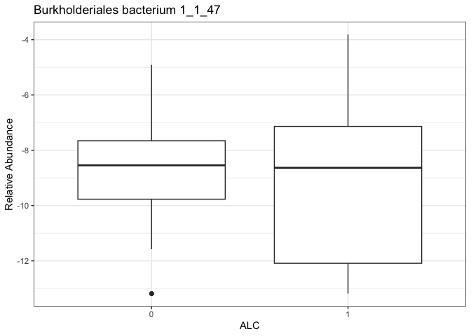
data("Dietary")
dat = Dietary
taxa_num = 100
dat$taxa_name[taxa_num] # taxa name
#> OTU100
#> "Burkholderiales bacterium 1_1_47"
W = dat$OTU[,taxa_num] # taxa count
M = dat$M # sequencing depth
ggplot(NULL)+
geom_boxplot(aes(
x = as.factor(dat$COV$ALC01),y=log((W+0.5)/M)))+
labs(title = dat$taxa_name[taxa_num],
x = 'ALC',y='Relative Abundance')+
theme_bw()
Use function ZIPG_main() to run our ZIPG model.
Input :
W : Observed taxa count data.
M : Sequencing depth, ZIPG use log(M) as offset by
default.
X, X_star : Covariates of interesting of
differential abundance and differential varibility, input as
formula.
Output list:
ZIPG_res$init : pscl results, used as
initialization.
ZIPG_res$res : ZIPG output evaluated at last EM
iteration.
ZIPG_res$res$par : ZIPG estimation for \(\Omega = (\beta,\beta^*,\gamma)\).
ZIPG_res$wald_test : ZIPG Wald test
ZIPG_res$logli : ZIPG log-likelihood
ZIPG_res <- ZIPG_main(data = dat$COV,
                      X = ~ALC01+nutrPC1+nutrPC2, X_star = ~ ALC01,
                      W = W, M = M)
res = ZIPG_summary(ZIPG_res)
#>           ZIPG Wald
#>        Estimation     SE     pval
#> beta0      -7.371 0.1512 0.00e+00 ***
#> beta1       0.121 0.1985 5.41e-01
#> beta2       0.106 0.0188 1.41e-08 ***
#> beta3      -0.118 0.0287 4.17e-05 ***
#> beta0*      0.525 0.1199 1.20e-05 ***
#> beta1*      0.606 0.1406 1.63e-05 ***
#> gamma -2.080 0.1460 4.93e-46 ***Set the bootstrap replicates B in
bWald_list to conduct ZIPG-bWald, results and covariance
matrix can be find in ZIPG_res$bWald.
set.seed(123)
# Set bootstrap replicates B
bWald_list = list(B = 100)
# Wait for a wile
ZIPG_res1 = ZIPG_main(
  data = dat$COV,
  X = ~ALC01+nutrPC1+nutrPC2, X_star = ~ ALC01,
  W = W, M = M,
  bWald_list = bWald_list)
#> Running non-parametric bootstrap wald test
#> Finish
res = ZIPG_summary(ZIPG_res1,type = 'bWald')
#>           ZIPG bWald
#>        Estimation     SE     pval
#> beta0      -7.371 0.1896 0.00e+00 ***
#> beta1       0.121 0.2323 6.01e-01
#> beta2       0.106 0.0209 3.51e-07 ***
#> beta3      -0.118 0.0342 5.95e-04 ***
#> beta0*      0.525 0.1283 4.30e-05 ***
#> beta1*      0.606 0.1740 4.97e-04 ***
#> gamma      -2.080 0.3698 1.86e-08 ***
res = ZIPG_CI(ZIPG_res1,type='bWald',alpha = 0.05)
#>         ZIPG Wald Confidence interval
#>        Estimation      lb      ub
#> beta0      -7.371 -7.7421 -6.9990
#> beta1       0.121 -0.3338  0.5768
#> beta2       0.106  0.0655  0.1474
#> beta3      -0.118 -0.1847 -0.0505
#> beta0*      0.525  0.2734  0.7765
#> beta1*      0.606  0.2649  0.9470
#> gamma      -2.080 -2.8046 -1.3551
To test more complicated hypothesis, you may use the covariance matirx driven from bootstrap.
round(ZIPG_res1$bWald$vcov,3)
#>        [,1]   [,2]   [,3]   [,4]   [,5]   [,6]   [,7]
#> [1,]  0.036 -0.040  0.001  0.003  0.005 -0.009  0.013
#> [2,] -0.040  0.054 -0.001 -0.004 -0.006  0.009 -0.008
#> [3,]  0.001 -0.001  0.000  0.000  0.000  0.001 -0.001
#> [4,]  0.003 -0.004  0.000  0.001  0.001 -0.002  0.003
#> [5,]  0.005 -0.006  0.000  0.001  0.016 -0.014 -0.012
#> [6,] -0.009  0.009  0.001 -0.002 -0.014  0.030 -0.025
#> [7,] 0.013 -0.008 -0.001 0.003 -0.012 -0.025 0.137Set bootstrap replicates B and the null hypothesis by
formula X0 and X_star0 in
pbWald_list to conduct ZIPG-pbWald, results can be find in
ZIPG_res$pbWald
# test beta1star, the 6th parameter
#
pbWald_list = list(
  X0 = ~ALC01 + nutrPC1+nutrPC2,
  X_star0 = ~ 1,
  B = 100
)

ZIPG_res2 = ZIPG_main(
  data = dat$COV,
  X = ~ALC01+nutrPC1+nutrPC2, X_star = ~ ALC01,
  W = W, M = M,
  pbWald_list= pbWald_list)
#> Running parametric bootstrap wald test
#> Finish

res = ZIPG_summary(ZIPG_res2,type ='pbWald')
#>    ZIPG pbWald
#>  H0: beta1* = 0
#> pvalue = 0.0099These binaries (installable software) and packages are in development.
They may not be fully stable and should be used with caution. We make no claims about them.
Health stats visible at Monitor.