The hardware and bandwidth for this mirror is donated by dogado GmbH, the Webhosting and Full Service-Cloud Provider. Check out our Wordpress Tutorial.
If you wish to report a bug, or if you are interested in having us mirror your free-software or open-source project, please feel free to contact us at mirror[@]dogado.de.
![]()
The TVMVP package implements a method of estimating a time dependent covariance matrix based on time series data using principal component analysis on kernel weighted data. The package also includes a hypothesis test of time-invariant covariance, and methods for implementing the time-dependent covariance matrix in a portfolio optimization setting. This package is an R implementation of the method proposed in Fan et al. (2024). The original authors provide a Matlab implementation at https://github.com/RuikeWu/TV-MVP.
The local PCA method, method for determining the number of factors, and associated hypothesis test are based on Su and Wang (2017). The approach to time-varying portfolio optimization follows Fan et al. (2024). The regularisation applied to the residual covariance matrix adopts the technique introduced by Chen et al. (2019).
You can install the development version of TVMVP from GitHub with:
devtools::install_gitbub("erilill/TV-MVP")provided that the package “devtools” has been installed beforehand.
After installing the package, you attach the package by running the code:
library(TVMVP)For this example we will use simulated data, however most use cases for this package will be using financial data. This can be accessed using one of the many API’s available in R and elsewhere.
set.seed(123)
uT <- 100  # Number of time periods
up <- 20   # Number of assets
returns <- matrix(rnorm(uT * up, mean = 0.001, sd = 0.02), ncol = up)
For this example we will give usage examples using the methods of the
R6 class TVMVP, and a brief example of how to use the
functions if this is your preferred method of implementation
We start by initializing the object of class TVMVP and
set the data:
tvmvp_obj <- TVMVP$new()
tvmvp_obj$set_data(returns)
#> ℹ data set "16.22 kB" with 100 rows and 20 columns
Then we determine the number of factors and conduct the hypothesis test:
tvmvp_obj$determine_factors(max_m=5)
#> ! use default Silverman bandwidth
#> ℹ using max_m = 5 and bandwidth = 0.200158593074818
#> [1] 1
tvmvp_obj$get_optimal_m()
#> [1] 1

tvmvp_obj$hyptest(iB=10) # Use larger iB in practice
#> Computing ■■■■■■■ 20% | ETA: 8s
#> Computing ■■■■■■■■■■                        30% | ETA:  7sComputing ■■■■■■■■■■■■■                     40% | ETA:  6sComputing ■■■■■■■■■■■■■■■■                  50% | ETA:  5sComputing ■■■■■■■■■■■■■■■■■■■               60% | ETA:  4sComputing ■■■■■■■■■■■■■■■■■■■■■■            70% | ETA:  3sComputing ■■■■■■■■■■■■■■■■■■■■■■■■■         80% | ETA:  2sComputing ■■■■■■■■■■■■■■■■■■■■■■■■■■■■      90% | ETA:  1s                                                           J_pT = 34.7556, p-value = 0.0000: Strong evidence that the covariance is time-varying.
tvmvp_obj
#> ℹ Object of TVMVP
#> data set "16.22 kB" with 100 rows and 20 columns
#> - bandwidth = 0.200158593074818
#> - max_m = 5
#> - optimal_m = 1
#> - test statistic = 34.7556191258208 with bootstrap p-value = 0
#>   run `get_optimal_m()`
The function determine_factors uses a BIC-type
information criterion in order to determine the optimal number of
factors to be used in the model. More information can be seen in section
2.2 of the thesis. The input variables are the data matrix
returns, the max number of factors to be tested
max_m, and the bandwidth to be used bandwidth.
The package offers the functionality of computing the bandwidth using
Silverman’s rule of thumb with the function silverman(),
however other methods could be used. The function outputs the optimal
number of factors optimal_m, and the values of the
information criteria for the different number of factors
IC_values.
hyptest implements the hypothesis test of constant
factor loadings introduced by Su & Wong (2017). Under some
conditions, the test statistic \(J\)
follows a standard normal distribution under the null. However, the test
have been proven to be somewhat unreliable in finite sample usage, which
is why the option of computing a bootstrap p-value is included. More
information can be found in section 2.3 in the thesis. The function take
the input: a data matrix of multiple time series returns,
the number of factors m, the number of bootstrap
replications iB, and the kernel function
kernel_func. The package offers the Epanechnikov kernel,
however others could also be used.
The next step, and the most relevant functionality is the portfolio
optimization. The package offers two functions for this purpose:
expanding_tvmvp which implements a expanding window in
order to evaluate the performance of a minimum variance portfolio
implemented using the time-varying covariance matrix, and
predict_portfolio which implements an out of sample
prediction of the portfolio.
Note that these functions expect log returns and log risk free rate.
mvp_result <- tvmvp_obj$expanding_tvmvp(
  initial_window = 60,
  rebal_period   = 5,
  max_factors    = 10,
  return_type    = "daily",
  rf             = NULL
)

mvp_result
#>
#> ── Expanding Window Portfolio Analysis ─────────────────────────────────────────
#> ────────────────────────────────────────────────────────────────────────────────
#>
#> ── Summary Metrics ──
#>
#>            Method       CER         MER          SD        SR   MER_ann
#>  Time-Varying MVP 0.1491042 0.003727605 0.008475585 0.4398050 0.9393564
#>      Equal Weight 0.1382776 0.003456941 0.004270192 0.8095516 0.8711491
#>      SD_ann
#>  0.13454575
#>  0.06778719
#> ────────────────────────────────────────────────────────────────────────────────
#> ── Detailed Components ──
#>
#> The detailed portfolio outputs are stored in the following elements:
#> - Time-Varying MVP: Access via `$TVMVP`
#> - Equal Weight: Access via `$Equal`
plot(mvp_result)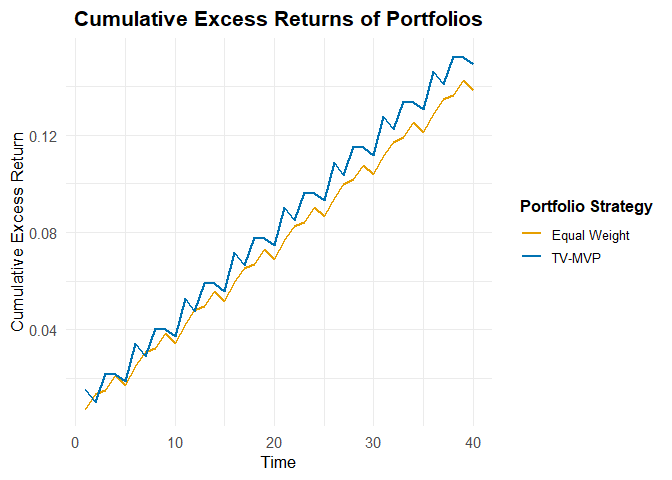
The expanding_tvmvp function takes the input:
returns a \(T\times p\)
data matrix, initial_window which is the initial holding
window used for estimation, rebal_period which is the
length of the rebalancing period to be used in the evaluation,
max_factors used in the determination of the optimal number
of factors, return_type can be set to “daily”, “weekly”,
and “monthly”, and is used for annualization of the results,
kernel_func, and rf which denotes the risk
free rate, this can be input either as a scalar or at \((T-initialwindow)\times 1\) numerical
vector. The function outputs relevant metrics for evaluation of the
performance of the portfolio such as cumulative excess returns, standard
deviation, and Sharpe ratio.
prediction <- tvmvp_obj$predict_portfolio(horizon = 21, min_return = 0.5,
                                   max_SR = TRUE)
prediction
#>
#> ── Portfolio Optimization Predictions ──────────────────────────────────────────
#> ────────────────────────────────────────────────────────────────────────────────
#>
#> ── Summary Metrics ──
#>
#>                        Method expected_return       risk    sharpe
#>    Minimum Variance Portfolio      0.03355982 0.01843029 0.3973543
#>          Maximum SR Portfolio      0.06666808 0.02597654 0.5600503
#>  Return-Constrained Portfolio      0.50000000 0.25855695 0.4219919
#> ────────────────────────────────────────────────────────────────────────────────
#> ── Detailed Components ──
#>
#> The detailed portfolio outputs are stored in the following elements:
#> - MVP: Use object$MVP
#> - Maximum Sharpe Ratio Portfolio: Use object$max_SR
#> - Minimum Variance Portfolio with Return Constraint: Use object$MVPConstrained
weights <- prediction$getWeights("MVP")
The predict_portfolio functions makes out of sample
predictions of the portfolio performance. The functions offers three
different methods of portfolio optimization: Minimum variance, Minimum
variance with minimum returns constraint, and maximum Sharpe ratio
portfolio. The minimum variance portfolio is the default portfolio and
will always be computed when running this function. The minimum returns
constraint is set by imputing some min_return-value when
running the function, important to note is that the minimum return
constraint is set for the entire horizon and is not a daily constraint.
The maximum SR portfolio is computed when max_SR is set to
TRUE.
If the pre-built functions does not fit your purpose, you can utilize the covariance function by running:
cov_mat <- tvmvp_obj$time_varying_cov()Which outputs the covariance matrix weighted around the last observation in returns.
Below you see an example of how to use the functions instead:
# Determine number of factors
m <- determine_factors(returns = returns, max_m = 10, bandwidth = silverman(returns))$optimal_m
m

# Run test of constant loadings
hypothesis_test <- hyptest(returns = returns,
                            m = m,
                            B = 10, # Use larger B in practice
                            )

# Expanding window evaluation
mvp_result <- expanding_tvmvp(
  obj            = tvmvp_obj,
  initial_window = 60,
  rebal_period   = 5,
  max_factors    = 10,
  return_type    = "daily",
  kernel_func    = epanechnikov_kernel,
  rf             = 1e-04
)
mvp_result

# Optimize weights and predict performance out-of-sample
prediction <- predict_portfolio(obj = tvmvp_obj,
                                horizon = 21,
                                m = 10,
                                kernel_func = epanechnikov_kernel,
                                min_return=0.5,
                                max_SR = TRUE,
                                rf = 1e-04)
prediction
weights <- prediction$getWeights("MVP")

# For custom portfolio optimization, compute the time dependent covariance:
cov_mat <- time_varying_cov(obj = tvmvp_obj,
                            max_factors = 5,
                            bandwidth = silverman(returns),
                            kernel_func = epanechnikov_kernel,
                            M0 = 10,
                            rho_grid = seq(0.005, 2, length.out = 30),
                            floor_value = 1e-12,
                            epsilon2 = 1e-6,
                            full_output = FALSE)
These have the same functionality as the methods, however using the class methods is neater as the necessary parameters are cached in the object.
Lillrank, E. (2025). A Time-Varying Factor Approach to Covariance Estimation.
Su, L., & Wang, X. (2017). On time-varying factor models: Estimation and testing. Journal of Econometrics, 198(1), 84–101.
Fan, Q., Wu, R., Yang, Y., & Zhong, W. (2024). Time-varying minimum variance portfolio. Journal of Econometrics, 239(2), 105339.
Chen, J., Li, D., & Linton, O. (2019). A new semiparametric estimation approach for large dynamic covariance matrices with multiple conditioning variables. Journal of Econometrics, 212(1), 155–176.
These binaries (installable software) and packages are in development.
They may not be fully stable and should be used with caution. We make no claims about them.
Health stats visible at Monitor.