The hardware and bandwidth for this mirror is donated by dogado GmbH, the Webhosting and Full Service-Cloud Provider. Check out our Wordpress Tutorial.
If you wish to report a bug, or if you are interested in having us mirror your free-software or open-source project, please feel free to contact us at mirror[@]dogado.de.
The goal of SSOSVM is to use R to allow batch and online training of soft-margin support vector machines (SVMs). The training of SVMs usually requires that the data be available all at once in a single batch, however the Stochastic majorization-minimization (SMM) algorithm framework allows for the training of SVMs on streamed data instead http://doi.org/10.1007/s42081-018-0001-y. This package utilizes the SMM framework to provide functions for training SVMs with hinge loss, squared-hinge loss, and logistic loss, functions.
You can install SSOSVM from github with:
# install.packages("devtools")
devtools::install_github("andrewthomasjones/SSOSVM")Here is a very simple example using simulated data:
#setup
library(SSOSVM)
library(ggplot2)
#> Warning: package 'ggplot2' was built under R version 4.4.1

#simulations
sims <- generateSim(100, DELTA=3)

#fit using various loss functions
sq1<-SVMFit(sims$YMAT,"square")
h1<-SVMFit(sims$YMAT,"hinge")
l1<-SVMFit(sims$YMAT,"logistic")

#plot results
plot<-ggplot(data.frame(sims$YMAT), aes(colour=factor(YY), x=V2, y=V3))
plot<-plot+geom_point()+theme_bw()+xlab("X")+ylab("Y")+guides(colour=FALSE)
#> Warning: The `<scale>` argument of `guides()` cannot be `FALSE`. Use "none" instead as
#> of ggplot2 3.3.4.
#> This warning is displayed once every 8 hours.
#> Call `lifecycle::last_lifecycle_warnings()` to see where this warning was
#> generated.
plot<-plot+geom_abline(intercept=sq1$THETA[1],
                       slope=sq1$THETA[2]/sq1$THETA[3], colour="blue")
plot<-plot+geom_abline(intercept=h1$THETA[1],
                       slope=h1$THETA[2]/h1$THETA[3], colour="green")
plot<-plot+geom_abline(intercept=l1$THETA[1],
                       slope=l1$THETA[2]/l1$THETA[3], colour="red")
plot
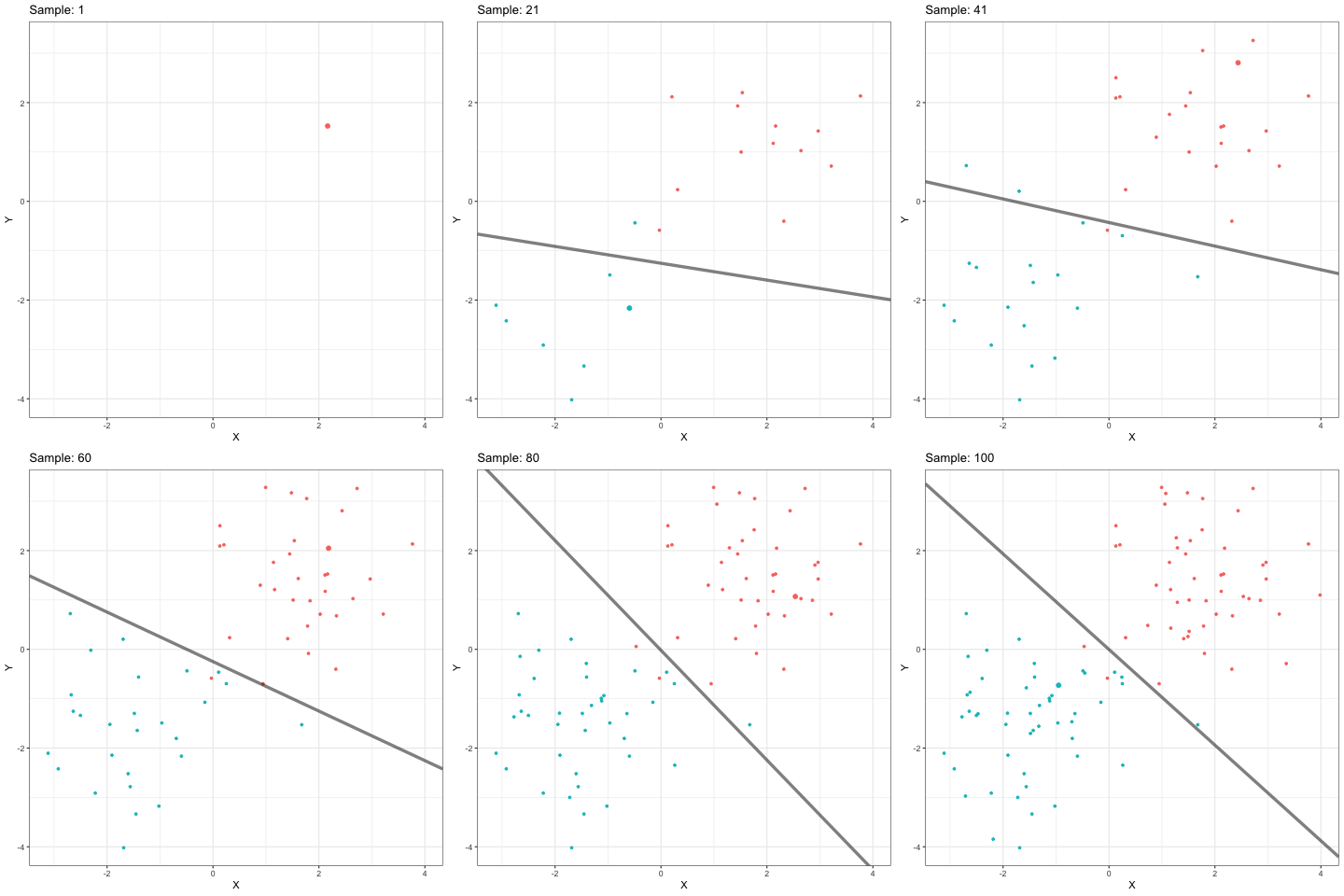
Here is an animated example to demostrate the online nature of of the SSOSVM method:
library(ggplot2)
library(gganimate)

#set up
sims <- generateSim(10^2, DELTA=1.5)

#fit using various loss functions
sq1<-SVMFit(sims$YMAT,"square", returnAll = TRUE)
h1<-SVMFit(sims$YMAT,"hinge", returnAll = TRUE)
l1<-SVMFit(sims$YMAT,"logistic", returnAll = TRUE)

#dataframe
data<-data.frame(sample=1:10^2,
                 sims$YMAT,
                 logistic_int=l1$THETA_list[,1],
                 square_int=sq1$THETA_list[,1],
                 hinge_int=h1$THETA_list[,1],
                 logistic_sl=l1$THETA_list[,2]/l1$THETA_list[,3],
                 square_sl=sq1$THETA_list[,2]/sq1$THETA_list[,3],
                 hinge_sl=h1$THETA_list[,2]/h1$THETA_list[,3])

#base plot
plot<-ggplot(data, aes(colour=factor(YY), x=V2, y=V3))+
  geom_point(size=2)+theme_bw()+xlab("X")+ylab("Y")+
  guides(colour=FALSE)+geom_abline(size=1.6,alpha=.5, aes(intercept=square_int, slope=square_sl))

#animate
example <- plot + transition_time(sample)+
  labs(title =  "Sample: {frame_time}")+
  shadow_mark(alpha = 1, size = 1, exclude_layer = 2)

#save animation
anim_save("./inst/example.gif", example, fps=2.5)
These binaries (installable software) and packages are in development.
They may not be fully stable and should be used with caution. We make no claims about them.
Health stats visible at Monitor.