The hardware and bandwidth for this mirror is donated by dogado GmbH, the Webhosting and Full Service-Cloud Provider. Check out our Wordpress Tutorial.
If you wish to report a bug, or if you are interested in having us mirror your free-software or open-source project, please feel free to contact us at mirror[@]dogado.de.
![]()
![]()
Chest pain? Calculate your cardiovascular risk score.
The goal of RiskScorescvd R package is to calculate the most commonly used cardiovascular risk scores. Original research publication can be found here: https://openheart.bmj.com/content/11/2/e002755
We have developed nine of the most commonly used risk scores with a dependency (ASCVD [PooledCohort]) making the following available:
NOTE: Troponin I values should be used. Additional functions for Troponin T are under development
You can install from CRAN with:
# Install from CRAN
install.packages("RiskScorescvd")
You can install the development version of RiskScorescvd from GitHub with:
# install.packages("devtools")
devtools::install_github("dvicencio/RiskScorescvd")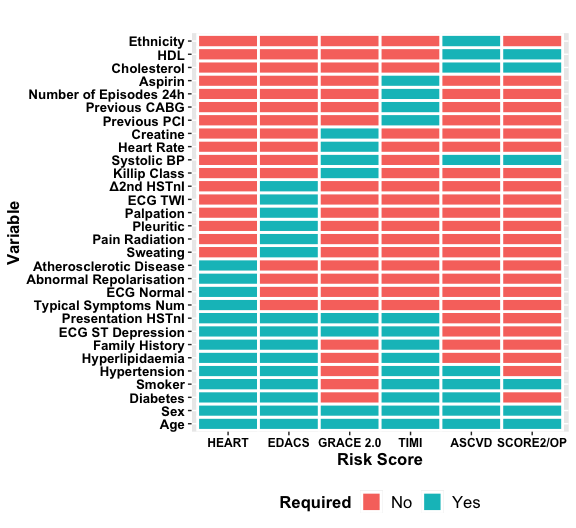
This is a basic example of how the data set should look to calculate all risk scores available in the package:
library(RiskScorescvd)
#> Loading required package: PooledCohort
# Create a data frame or list with the necessary variables
 # Set the number of rows
 num_rows <- 100

 # Create a large dataset with 100 rows
  cohort_xx <- data.frame(
   typical_symptoms.num = as.numeric(sample(0:6, num_rows, replace = TRUE)),
   ecg.normal = as.numeric(sample(c(0, 1), num_rows, replace = TRUE)),
   abn.repolarisation = as.numeric(sample(c(0, 1), num_rows, replace = TRUE)),
   ecg.st.depression = as.numeric(sample(c(0, 1), num_rows, replace = TRUE)),
   Age = as.numeric(sample(30:80, num_rows, replace = TRUE)),
   diabetes = sample(c(1, 0), num_rows, replace = TRUE),
   smoker = sample(c(1, 0), num_rows, replace = TRUE),
   hypertension = sample(c(1, 0), num_rows, replace = TRUE),
   hyperlipidaemia = sample(c(1, 0), num_rows, replace = TRUE),
   family.history = sample(c(1, 0), num_rows, replace = TRUE),
   atherosclerotic.disease = sample(c(1, 0), num_rows, replace = TRUE),
   presentation_hstni = as.numeric(sample(10:100, num_rows, replace = TRUE)),
   Gender = sample(c("male", "female"), num_rows, replace = TRUE),
   sweating = as.numeric(sample(c(0, 1), num_rows, replace = TRUE)),
   pain.radiation = as.numeric(sample(c(0, 1), num_rows, replace = TRUE)),
   pleuritic = as.numeric(sample(c(0, 1), num_rows, replace = TRUE)),
   palpation = as.numeric(sample(c(0, 1), num_rows, replace = TRUE)),
   ecg.twi = as.numeric(sample(c(0, 1), num_rows, replace = TRUE)),
   second_hstni = as.numeric(sample(1:200, num_rows, replace = TRUE)),
   killip.class = as.numeric(sample(1:4, num_rows, replace = TRUE)),
   heart.rate = as.numeric(sample(0:300, num_rows, replace = TRUE)),
   systolic.bp = as.numeric(sample(40:300, num_rows, replace = TRUE)),
   aspirin = as.numeric(sample(c(0, 1), num_rows, replace = TRUE)),
   creat = as.numeric(sample(0:4, num_rows, replace = TRUE)),
   number.of.episodes.24h = as.numeric(sample(0:20, num_rows, replace = TRUE)),
   previous.pci = as.numeric(sample(c(0, 1), num_rows, replace = TRUE)),
   cardiac.arrest = as.numeric(sample(c(0, 1), num_rows, replace = TRUE)),
   previous.cabg = as.numeric(sample(c(0, 1), num_rows, replace = TRUE)),
   total.chol = as.numeric(sample(5:100, num_rows, replace = TRUE)),
   total.hdl = as.numeric(sample(2:5, num_rows, replace = TRUE)),
   Ethnicity = sample(c("white", "black", "asian", "other"), num_rows, replace = TRUE),
   eGFR = as.numeric(sample(15:120, num_rows, replace = TRUE)),
   ACR = as.numeric(sample(5:1500, num_rows, replace = TRUE)),
   trace = sample(c("trace", "1+", "2+", "3+", "4+"), num_rows, replace = TRUE)
 )

  str(cohort_xx)
#> 'data.frame':    100 obs. of  34 variables:
#>  $ typical_symptoms.num   : num  1 1 0 2 4 6 6 2 4 4 ...
#>  $ ecg.normal             : num  0 1 1 0 0 0 0 1 1 0 ...
#>  $ abn.repolarisation     : num  1 0 1 1 0 0 0 1 0 1 ...
#>  $ ecg.st.depression      : num  0 1 0 1 1 0 1 0 1 0 ...
#>  $ Age                    : num  61 75 60 44 47 46 71 39 56 50 ...
#>  $ diabetes               : num  1 1 1 1 0 1 0 0 1 1 ...
#>  $ smoker                 : num  0 1 0 1 0 0 1 1 1 1 ...
#>  $ hypertension           : num  1 1 1 1 1 0 1 0 0 0 ...
#>  $ hyperlipidaemia        : num  1 0 1 0 1 0 0 1 1 0 ...
#>  $ family.history         : num  1 0 0 0 1 1 0 1 0 1 ...
#>  $ atherosclerotic.disease: num  1 1 1 0 1 0 0 1 1 0 ...
#>  $ presentation_hstni     : num  19 75 96 76 82 35 36 20 54 27 ...
#>  $ Gender                 : chr  "male" "female" "male" "female" ...
#>  $ sweating               : num  1 0 0 1 1 0 1 0 1 0 ...
#>  $ pain.radiation         : num  1 1 1 1 1 1 1 1 0 1 ...
#>  $ pleuritic              : num  1 1 0 0 0 1 1 1 0 0 ...
#>  $ palpation              : num  1 0 1 0 0 0 0 0 0 1 ...
#>  $ ecg.twi                : num  0 1 1 0 0 1 1 0 0 1 ...
#>  $ second_hstni           : num  157 131 58 45 174 23 178 189 20 78 ...
#>  $ killip.class           : num  3 4 4 3 2 3 2 2 1 4 ...
#>  $ heart.rate             : num  227 273 122 169 147 291 267 266 198 148 ...
#>  $ systolic.bp            : num  41 218 153 118 282 92 191 293 101 267 ...
#>  $ aspirin                : num  1 0 0 1 0 0 1 0 1 1 ...
#>  $ creat                  : num  3 3 2 3 3 0 1 2 4 3 ...
#>  $ number.of.episodes.24h : num  11 12 19 18 12 17 10 16 4 8 ...
#>  $ previous.pci           : num  0 0 0 1 0 1 0 1 1 0 ...
#>  $ cardiac.arrest         : num  0 1 0 0 1 1 0 0 1 1 ...
#>  $ previous.cabg          : num  0 1 1 0 0 0 0 1 0 0 ...
#>  $ total.chol             : num  97 89 52 93 29 56 58 99 91 40 ...
#>  $ total.hdl              : num  3 3 4 3 4 5 5 4 5 2 ...
#>  $ Ethnicity              : chr  "other" "white" "white" "white" ...
#>  $ eGFR                   : num  77 69 110 81 22 76 68 58 43 65 ...
#>  $ ACR                    : num  782 1161 1005 595 840 ...
#> $ trace : chr "trace" "4+" "4+" "trace" ...This is a basic example of how to calculate all risk scores available in the package and create a new data set with 12 new variables of the calculated and classified risk scores:
# Call the function with the cohort_xx to calculate all risk scores available in the package
new_data_frame <- calc_scores(data = cohort_xx)

# Select columns created after calculation
All_scores <- new_data_frame %>% select(HEART_score, HEART_strat, EDACS_score, EDACS_strat, GRACE_score, GRACE_strat, TIMI_score, TIMI_strat, SCORE2_score, SCORE2_strat, ASCVD_score, ASCVD_strat)

# Observe the results
head(All_scores)
#> # A tibble: 6 × 12
#> # Rowwise:
#>   HEART_score HEART_strat   EDACS_score EDACS_strat  GRACE_score GRACE_strat
#>         <dbl> <ord>               <dbl> <ord>              <dbl> <ord>
#> 1           4 Moderate risk          14 Not low risk         150 High risk
#> 2           8 High risk              15 Not low risk         181 High risk
#> 3           5 Moderate risk          13 Not low risk         132 High risk
#> 4           7 High risk              14 Not low risk         131 High risk
#> 5           8 High risk              16 Not low risk          88 Low risk
#> 6           6 Moderate risk           5 Not low risk         132 High risk
#> # ℹ 6 more variables: TIMI_score <dbl>, TIMI_strat <ord>, SCORE2_score <dbl>,
#> #   SCORE2_strat <ord>, ASCVD_score <dbl>, ASCVD_strat <ord>

# Create a summary of them to obtain an initial idea of distribution
summary(All_scores)
#>   HEART_score           HEART_strat  EDACS_score          EDACS_strat
#>  Min.   : 2.00   Low risk     : 6   Min.   :-2.00   Low risk    : 1
#>  1st Qu.: 5.00   Moderate risk:54   1st Qu.: 5.00   Not low risk:99
#>  Median : 6.00   High risk    :40   Median :10.00
#>  Mean   : 6.06                      Mean   :10.78
#>  3rd Qu.: 7.00                      3rd Qu.:16.00
#>  Max.   :10.00                      Max.   :30.00
#>   GRACE_score            GRACE_strat   TIMI_score           TIMI_strat
#>  Min.   : 29.00   Low risk     :30   Min.   :2.00   Very low risk: 0
#>  1st Qu.: 85.75   Moderate risk:34   1st Qu.:4.00   Low risk     : 6
#>  Median :107.00   High risk    :36   Median :4.00   Moderate risk:49
#>  Mean   :108.53                      Mean   :4.44   High risk    :45
#>  3rd Qu.:132.00                      3rd Qu.:5.00
#>  Max.   :205.00                      Max.   :7.00
#>   SCORE2_score           SCORE2_strat  ASCVD_score            ASCVD_strat
#>  Min.   :  0.00   Very low risk: 0    Min.   :0.0000   Very low risk: 7
#>  1st Qu.: 55.00   Low risk     : 6    1st Qu.:0.1900   Low risk     : 2
#>  Median :100.00   Moderate risk: 6    Median :0.4650   Moderate risk:17
#>  Mean   : 75.87   High risk    :88    Mean   :0.5027   High risk    :74
#>  3rd Qu.:100.00                       3rd Qu.:0.8300
#>  Max.   :100.00                       Max.   :1.0000
These binaries (installable software) and packages are in development.
They may not be fully stable and should be used with caution. We make no claims about them.
Health stats visible at Monitor.