The hardware and bandwidth for this mirror is donated by dogado GmbH, the Webhosting and Full Service-Cloud Provider. Check out our Wordpress Tutorial.
If you wish to report a bug, or if you are interested in having us mirror your free-software or open-source project, please feel free to contact us at mirror[@]dogado.de.
![]()
Ten C++ functions are exposed by this package:
std::string rgb2hex(double r, double g, double b);
std::string rgba2hex(double r, double g, double b, double a);
std::string hsluv2hex(double h, double s, double l);
std::string hsluv2hex(double h, double s, double l, double alpha);
std::string hsv2hex(double h, double s, double v);
std::string hsv2hex(double h, double s, double v, double alpha);
std::string hsl2hex(double h, double s, double l);
std::string hsl2hex(double h, double s, double l, double alpha);
std::string hsi2hex(double h, double s, double i);
std::string hsi2hex(double h, double s, double i, double alpha);
r, g, b ∈ [0, 255] (red, green, blue)
a, alpha ∈ [0, 1] (opacity)
h ∈ [0, 360] (hue)
s,l,v,i ∈ [0, 100] (saturation, lightness, value, intensity)
The LinkingTo field in the DESCRIPTION file should look like
LinkingTo:
    Rcpp,
    RcppColors
Then, in your C++ file, you can call the above functions like this:
#include <RcppColors.h>

std::string mycolor = RcppColors::rgb2hex(0.0, 128.0, 255.0);Fourteen color maps are available in R.
library(RcppColors)
library(Bessel)
x <- y <- seq(-4, 4, len = 1500)
# complex grid
W <- outer(y, x, function(x, y) complex(real = x, imaginary = y))
# computes Bessel values
Z <- matrix(BesselY(W, nu = 3), nrow = nrow(W), ncol = ncol(W))
# maps them to colors
image <- colorMap1(Z)
# plot
opar <- par(mar = c(0,0,0,0), bg = "#15191E")
plot(
  c(-100, 100), c(-100, 100), type = "n",
  xlab = "", ylab = "", axes = FALSE, asp = 1
)
rasterImage(image, -100, -100, 100, 100)
par(opar)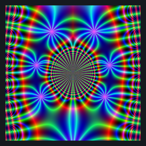
library(RcppColors)
library(Carlson)
library(rgl)
library(Rvcg)

mesh <- vcgSphere(subdivision = 8)

color <- apply(mesh$vb[-4L, ], 2L, function(xyz){
  if(sum(xyz == 0) >= 2){
    z <- NA_complex_
  }else{
    a <- xyz[1]
    b <- xyz[2]
    c <- xyz[3]
    z <- Carlson_RJ(a, b, c, 1i, 1e-5)
  }
  colorMap1(z)
})

mesh$material <- list(color = color)

open3d(windowRect = c(50, 50, 562, 562), zoom = 0.75)
bg3d("whitesmoke")
shade3d(mesh)
library(RcppColors)
library(jacobi)
library(rgl)
library(Rvcg)

mesh <- vcgSphere(subdivision = 8)

color <- apply(mesh$vb[-4L, ], 2L, function(xyz){
  a <- xyz[1]
  b <- xyz[2]
  c <- xyz[3]
  z <- wzeta(a + 1i* b, tau = (1i+c)/2)
  colorMap1(z)
})

mesh$material <- list(color = color)

open3d(windowRect = c(50, 50, 562, 562), zoom = 0.75)
bg3d("palevioletred2")
shade3d(mesh)
library(RcppColors)
ikeda <- Vectorize(function(x, y, tau0 = 0, gamma = 2.5){
  for(k in 1L:5L){
    tau <- tau0 - 6.0/(1.0 + x*x + y*y)
    newx <- 0.97 + gamma * (x*cos(tau) - y*sin(tau))
    y <- gamma * (x*sin(tau)+y*cos(tau))
    x <- newx
  }
  z <- complex(real = x, imaginary = y)
  colorMap1(z, reverse = c(TRUE, FALSE, FALSE))
})

x <- y <- seq(-3, 3, len = 3000)
image <- outer(y, x, function(x, y) ikeda(x, y))

opar <- par(mar = c(0,0,0,0), bg = "#002240")
plot(
  c(-100, 100), c(-100, 100), type = "n",
  xlab = "", ylab = "", axes = FALSE, asp = 1
)
rasterImage(image, -100, -100, 100, 100)
par(opar)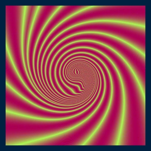
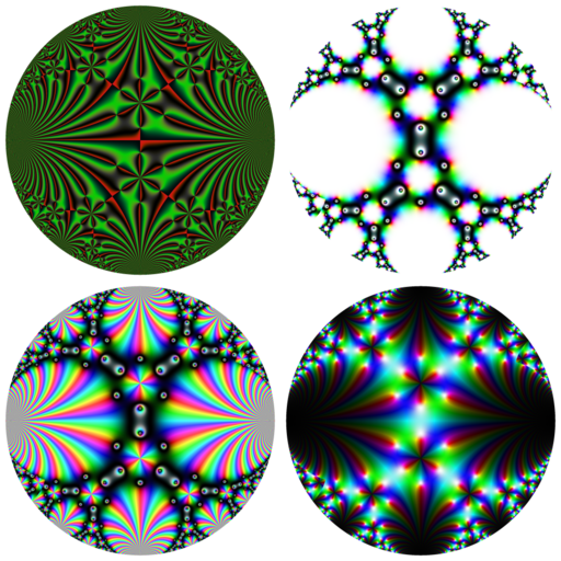
library(RcppColors)
library(jacobi)

f <- Vectorize(function(q){
  if(Mod(q) > 1  || (Im(q) == 0 && Re(q) <= 0)){
    z <- NA_complex_
  }else{
    z <- EisensteinE(6, q)
  }
  colorMap2(z, bkgcolor = "#002240")
})

x <- y <- seq(-1, 1, len = 2000)
image <- outer(y, x, function(x, y){
  f(complex(real = x, imaginary = y))
})

opar <- par(mar = c(0,0,0,0), bg = "#002240")
plot(
  c(-100, 100), c(-100, 100), type = "n",
  xlab = "", ylab = "", axes = FALSE, asp = 1
)
rasterImage(image, -100, -100, 100, 100)
par(opar)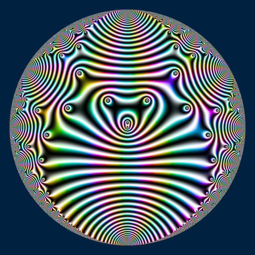
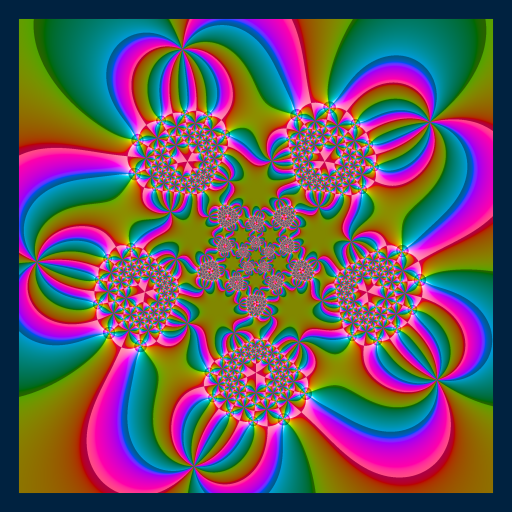
library(RcppColors)
library(jacobi)

f <- Vectorize(function(q){
  if(Mod(q) >= 1){
    NA_complex_
  }else{
    tau <- -1i * log(q) / pi
    if(Im(tau) <= 0){
      NA_complex_
    }else{
      kleinj(tau) / 1728
    }
  }
})

x <- y <- seq(-1, 1, len = 3000)
Z <- outer(y, x, function(x, y){
  f(complex(real = x, imaginary = y))
})
image <- colorMap2(1/Z, bkgcolor = "#002240", reverse = c(T,T,T))

opar <- par(mar = c(0,0,0,0), bg = "#002240")
plot(
  c(-100, 100), c(-100, 100), type = "n",
  xlab = "", ylab = "", axes = FALSE, asp = 1
)
rasterImage(image, -100, -100, 100, 100)
par(opar)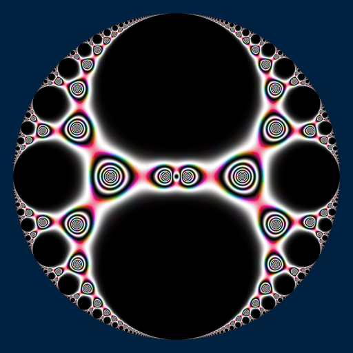
library(RcppColors)
library(jacobi)
library(rgl)
library(Rvcg)
library(pracma)

mesh <- vcgSphere(8)
sphcoords <- cart2sph(t(mesh$vb[-4L, ]))
theta <- sphcoords[, 1L] / pi
phi   <- sphcoords[, 2L] / pi * 2
Z <- wsigma(theta + 1i * phi, tau = 2+2i)
color <- colorMap1(Z, reverse = c(TRUE, FALSE, TRUE))
mesh$material <- list(color = color)

open3d(windowRect = c(50, 50, 562, 562), zoom = 0.75)
bg3d("lightgrey")
shade3d(mesh)
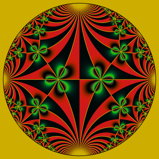
# Klein-Fibonacci map ####
library(jacobi)
library(RcppColors)

# the modified Cayley transformation
Phi <- function(z) (1i*z + 1) / (z + 1i)
PhiInv <- function(z) {
  1i + (2i*z) / (1i - z)
}
# background color
bkgcol <- "#ffffff"
# make the color mapping
f <- function(x, y) {
  z <- complex(real = x, imaginary = y)
  w <- PhiInv(z)
  ifelse(
    Mod(z) > 0.96,
    NA_complex_,
    ifelse(
      y < 0,
      -1/w, w
    )
  )
}
x <- seq(-1, 1, length.out = 2048)
y <- seq(-1, 1, length.out = 2048)
Z <- outer(x, y, f)
K <- kleinj(Z) / 1728
G <- K / (1 - K - K*K)
image <- colorMap4(G, bkgcolor = bkgcol)
# plot
opar <- par(mar = c(0,0,0,0), bg = bkgcol)
plot(
  c(-1, 1), c(-1, 1), type = "n",
  xlab = NA, ylab = NA, axes = FALSE, asp = 1
)
rasterImage(image, -1, -1, 1, 1)

# now we add the Dedekind tessellation (the white lines)
library(PlaneGeometry)
isInteger <- function(x) abs(x - floor(x)) < x * 1e-6
abline(h = 0, col = "white", lwd = 2)
N <- 150L
for(n in 1L:N) {
  if(isInteger(n/2) && ((n/2L) %% 2L == 1L)) {
    next
  }
  for(p in 1:n) {
    q <- sqrt(n*n - p*p + 4L)
    cases <- (isInteger(q) && isInteger(q/2) && (n %% 2L == 1L)) ||
      (isInteger(q) && isInteger(q/4) && (n %% 4L == 0L))
    if(cases) {
      circ <- Circle$new(center = c(q, p)/n, radius = 2/n)
      draw(circ, border = "white", lwd = 2)
      circ <- Circle$new(center = c(-q, p)/n, radius = 2/n)
      draw(circ, border = "white", lwd = 2)
      circ <- Circle$new(center = c(q, -p)/n, radius = 2/n)
      draw(circ, border = "white", lwd = 2)
      circ <- Circle$new(center = c(-q, -p)/n, radius = 2/n)
      draw(circ, border = "white", lwd = 2)
    }
  }
}
par(opar)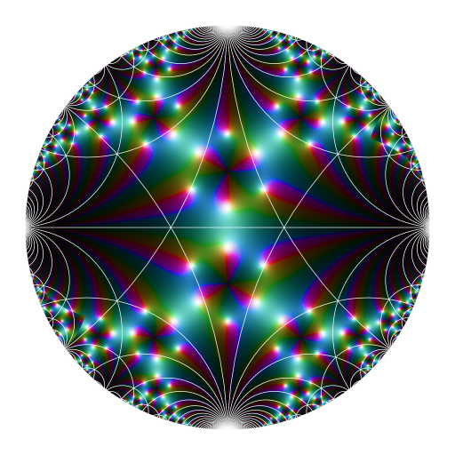
library(RcppColors)
library(jacobi)

f <- Vectorize(function(z){
  wsigma(z, omega = c(1, 0.25 + 1i))
})

x <- y <- seq(-5, 5, length.out = 512)
Z <- outer(y, x, function(x, y){
  f(complex(real = x, imaginary = y))
})

image <- colorMap5(Z, bkgcolor = "#002240")

opar <- par(mar = c(0,0,0,0), bg = "#002240")
plot(
  c(-100, 100), c(-100, 100), type = "n", xaxs="i", yaxs="i",
  xlab = NA, ylab = NA, axes = FALSE, asp = 1
)
rasterImage(image, -100, -100, 100, 100)
par(opar)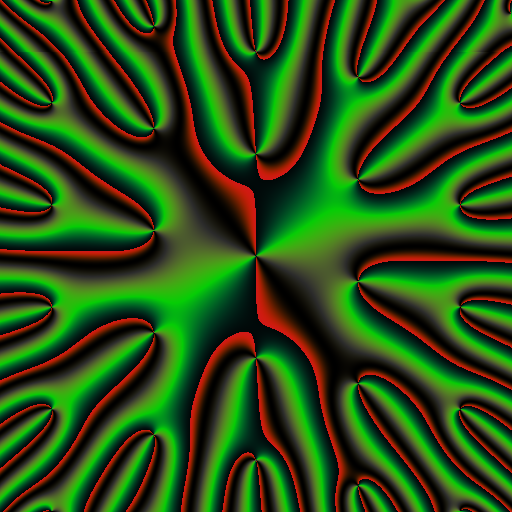
These binaries (installable software) and packages are in development.
They may not be fully stable and should be used with caution. We make no claims about them.
Health stats visible at Monitor.