The hardware and bandwidth for this mirror is donated by dogado GmbH, the Webhosting and Full Service-Cloud Provider. Check out our Wordpress Tutorial.
If you wish to report a bug, or if you are interested in having us mirror your free-software or open-source project, please feel free to contact us at mirror[@]dogado.de.
![]()
PopPsiSeqR is a package intended for analyzing the results of evolution & resequencing experiments. It builds on previous software published in @Earley2011. Offspring allele frequency spectrum is compared to the parental populations’ spectra and their expected equilibrium, in order to detect selected-for genomic regions.
You can install the development version of PopPsiSeqR from GitHub with:
# install.packages("pak")
pak::pak("csoeder/PopPsiSeqR")A table of allele frequencies is loaded and the frequency shift calculated:
library("PopPsiSeqR")

merged_frequencies.filename <- system.file("extdata",
  "merged_frequencies.example_data.tbl", package = "PopPsiSeqR")
merged_frequencies.bg <- import.freqtbl(merged_frequencies.filename)

frequency_shifts.bg <- freqShifter(merged_frequencies.bg)


head(frequency_shifts.bg %>% as.data.frame()
     %>% dplyr::select(-c(ends_with("_count"), ends_with("_deltaF"),  "name", "score"))
     %>% GenomicRanges::GRanges(), n=5)
#> GRanges object with 5 ranges and 10 metadata columns:
#>       seqnames    ranges strand |         ref         alt
#>          <Rle> <IRanges>  <Rle> | <character> <character>
#>   [1]    chr2L  10000208      * |           G           A
#>   [2]    chr2L  10000682      * |           T           C
#>   [3]    chr2L  10000709      * |           A           G
#>   [4]    chr2L  10000725      * |           G           A
#>   [5]    chr2L  10000933      * |           A           T
#>       selected_parent_alt_af backcrossed_parent_alt_af offspring_alt_af
#>                    <numeric>                 <numeric>        <numeric>
#>   [1]               0.277778                         0                0
#>   [2]               0.166667                         0                0
#>   [3]               0.250000                         0                0
#>   [4]               0.000000                         1                1
#>   [5]               0.000000                         1                1
#>         central mean_oriented_shift max_oriented_shift min_oriented_shift
#>       <numeric>           <numeric>          <numeric>          <numeric>
#>   [1] 0.1388890          -0.1388890           0.861111         -0.1388890
#>   [2] 0.0833335          -0.0833335           0.916667         -0.0833335
#>   [3] 0.1250000          -0.1250000           0.875000         -0.1250000
#>   [4] 0.5000000          -0.5000000           0.500000         -0.5000000
#>   [5] 0.5000000          -0.5000000           0.500000         -0.5000000
#>       AF_difference
#>           <numeric>
#>   [1]      0.277778
#>   [2]      0.166667
#>   [3]      0.250000
#>   [4]      1.000000
#>   [5]      1.000000
#>   -------
#>   seqinfo: 1 sequence from an unspecified genome; no seqlengths
The input data in this case is a table containing allele frequencies
for the selected and backcrossed parental population, and those of the
offspring population. This table was produced by joining the output of
VCFtools’ --freq utility, reformatted as BED files and
filtered to remove non-informative sites.
# calculating allele frequencies and converting to BED format
vcftools --vcf {input.vcf_in} --out {output.report_out} --freq;
cat {output.report_out}.frq | tail -n +2 | awk -v OFS='\\t' \
  '{{print $1,$2,$2+1,$4,$5,$6}}' > {output.frq_out}
# joining the frequency tables
bedtools intersect -wa -wb -a {input.slctd_frq} -b  {input.bckcrssd_frq} \
  | bedtools intersect -wa -wb -a - -b  {input.off_frq} \
  | cut -f 1,2,4-6,10,12,16,18 | tr ":" "\\t" \
  | awk -v OFS='\\t' '{{if(($6==$9) && ($9==$12) && ($7!=$10) )
  print $1,$2,$2+1,"0","0","+",$4,$6,$3,$7,$8,$10,$11,$13}}' \
  > {output.frqShft_out}.tmp
Once these frequencies have been collated, they can be loaded with
import.freqtbl(). The output can be easily written to disk
with export.freqshft(), where they can be averaged over
genomic intervals with utilities like bedtools map
bedtools makewindows -w {wildcards.window_size} -s {wildcards.slide_rate} -g {fai_path} -i winnum \
  | bedtools sort -i - > {output.windowed}

bedtools map -c 7,8,9,10,11,12,12 -o sum,sum,sum,sum,sum,sum,count -null NA -a {input.windows_in} \
  -b <( tail -n +2  {input.frqShft_in}   | cut -f  1-3,15-20 | nl -n ln  | \
  awk -v OFS='\t' '{{if( $5!="NA" && $6!="NA")print $2,$3,$4,$1,"0",".",$5,$6,$7,$8,$9,$10}}' \
  | bedtools sort -i - ) > {output.windowed_out}
These smoothed data can be reloaded with
import.smvshift(). A default plot of these smoothed data
can be produced with the windowedFrequencyShift.plotter()
function.
windowed_shifts.filename <- system.file("extdata", "windowed_shifts.example_data.bed",
  package = "PopPsiSeqR")

windowed_shifts.bg <- import.smvshift(windowed_shifts.filename, selected_parent = "sim",
  backcrossed_parent = "sech")

windowedFrequencyShift.plotter(windowed_shifts.bg,
  selected_parent = "sim", backcrossed_parent = "sech", main_title =
  "PopPsiSeq Results: offspring allele frequency\nrelative to neutral expectation, parental populations, and fixation")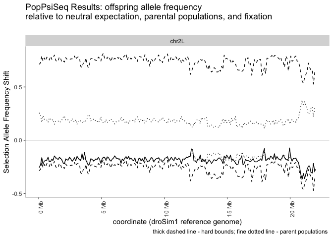
Finally, a simple comparison can be made between the results from
different experiments by calculating their arithmetic difference using
the subTractor() function:
lab_sechellia.filename <- system.file("extdata",
  "wild_sechellia.example_data.bed", package = "PopPsiSeqR")
lab.bg <- import.smvshift(lab_sechellia.filename)
lab.bg$sechellia <- "lab"


wild_sechellia.filename <- system.file("extdata",
  "lab_sechellia.example_data.bed", package = "PopPsiSeqR")
wild.bg <- import.smvshift(wild_sechellia.filename)
wild.bg$sechellia <- "wild"


sub.traction <- subTractor(lab.bg, wild.bg ,treament_name = "sechellia")

# autoplot(sub.traction, aes(y=lab_minus_wild), geom="line"
#   ) + labs(y="Difference in Allele Frequency Shift\n(lab - wild)",
#   title = "Difference between PopPsiSeq analyses based on lab-reared and wild-caught sechellia",
#   subtitle = "", caption ="",x= "coordinate (droSim1 reference genome)"
#   ) + theme_clear()
These binaries (installable software) and packages are in development.
They may not be fully stable and should be used with caution. We make no claims about them.
Health stats visible at Monitor.